Journal of Electromagnetic Analysis and Applications
Vol.06 No.12(2014), Article ID:50586,9 pages
10.4236/jemaa.2014.612038
Generalization of the Exact Solution of 1D Poisson Equation with Robin Boundary Conditions, Using the Finite Difference Method
Serigne Bira Gueye, Kharouna Talla, Cheikh Mbow
Département de Physique, Faculté des Sciences et Techniques, Université Cheikh Anta Diop, Dakar-Fann, Sénégal
Email: sbiragy@gmail.com
Copyright © 2014 by authors and Scientific Research Publishing Inc.
This work is licensed under the Creative Commons Attribution International License (CC BY).
http://creativecommons.org/licenses/by/4.0/


Received 8 August 2014; revised 2 September 2014; accepted 26 September 2014
ABSTRACT
A new and innovative method for solving the 1D Poisson Equation is presented, using the finite differences method, with Robin Boundary conditions. The exact formula of the inverse of the discretization matrix is determined. This is the first time that this famous matrix is inverted explicitly, without using the right hand side. Thus, the solution is determined in a direct, very accurate (O(h2)), and very fast (O(N)) manner. This new approach treats all cases of boundary conditions: Dirichlet, Neumann, and mixed. Therefore, it can serve as a reference for solving the Poisson equation in one dimension.
Keywords:
Robin Boundary, Poisson Equation, Matrix Inversion

1. Introduction
The Poisson equation is an elliptic differential equation well known and common to various scientific and technical domains such as physics, mathematics, chemistry, biology, etc. Its resolution generates a lot of interest to engineers, teachers, and researchers. Since, it allows analyzing in quantitative manner the studied phenomena: electrostatic, magnetostatic, wave propagation or heat diffusion in steady state. Many methods of resolution of this important equation exist, however, using the right hand side (RHS), for example, the method of Gaussian elimination or the Thomas algorithm.
Recently, a new method is proposed [1] [2] dealing with this equation in one dimensional case. This new approach, using the finite differences method (FDM), determined the inverse of the matrix obtained from algebraic equations. However, only the case of boundary conditions Dirichlet-Dirichlet (DD) [1] ; Neumann-Dirichlet (ND) and Dirichlet-Neumann (DN) [2] were treated.
The present study generalizes the solution of the Poisson equation and determines its solution for boundary conditions of third kind: Robin conditions. These mixed boundary conditions present a great interest in practice, because of combining two quantities: the function and its derivative. Here, a great innovation is that the solution is obtained in a very fast and precise way, and without using the RHS.
First, an inventory is made for possible cases of boundary conditions (DD) (DN), (ND), (RR), (RN), (NR), (DR) and (RD). Then, the cases, which must be solved are identified, considering that the first three cases of boundary problems have been solved in [1] and [2] . Then the cases (RR), (RN), (NR), were treated. The final solution is obtained, using an adequate choice of discretization, and inverting directly and exactly the discretization matrix. Thus, a numerical verification is done, considering a boundary problem of type (RR). The sensibility is determined, showing the predicated behavior of the truncation error and the very good accuracy of this new method. Finally, the cases of boundary conditions of type (DR) and (RD) are discussed and solved.
2. General Problem
The following boundary problem is to be solved:
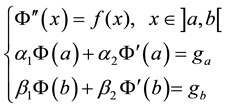 (1)
(1)
Here,  is, a scalar field, which depends on the real variable x. The function f(x) is a well known excitation and will be called the Right Hand Side (RHS) of the Poisson equation.
 ,
,  ,
,  , and
, and  are unknown values of
  and of its first derivative at points a and b, respectively. The reals
  and
and  are given constants. The coefficients
 ,
,  ,
,  , and
, and  are also known.
The type of boundary problem is given by the nature of the quadruplet ( ,
,  ,
,  ,
, ). For example (
 , 0,
, 0,  , 0) corresponds to a boundary problem of type Dirichlet-Dirichlet (DD), while the combination (0,
  ,
,  , 0) is for a boundary problem of type Neumann-Dirichlet (ND), etc.
Depending on the value of the quadruplet of coefficients, nine (9) boundary problems exist: (DD) (ND), (DN), (NN), (RR), (RN), (NR), (DR), and (RD). The first three problems (DD), (ND), and (DN) were solved in [1] and [2] . The problem (NN) leads to a non-regular discretization matrix.
This study will determine the solutions for all the remaining cases; and therefore can serve as reference for all that will involve the 1D Poisson equation. We distinguish three parts:
・  and
and . We will call this type of boundary problem Robin-Robin (RR). This part also covers Robin-Neumann (RN) and Neumann-Robin (NR) boundary problems. This is the most important part of this study because helping to resolve the next two parts.
・  and
and . This is the case of the Dirichlet-Robin (DR) boundary problem.
・  and
and . This is the case of the Robin-Dirichlet (RD) boundary problem.
3. 1D Poisson Equation with Robin-Robin (RR) Boundary Conditions
We consider the 1D Poisson equation with boundary conditions of type Robin-Robin (RR). This problem corresponds to the case, where  and
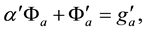
and . At points a and b, we have the following relations:
 , (2)
, (2)
where ,
,  ,
,  and
and 
We propose a new method of resolution of this problem. The latter requires a comfortable and adequate discretization as shown in Figure 1.

Figure 1. Discretization for Robin-Robin boundary conditions.
The mesh is composed of N + 2 points. N of them are in the interval of integration [a,b]. The other two are extra, additional, points [3] , [4] .
The mesh points  are defined by the following relation:
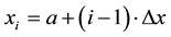 ,
,  , where
 designates the step size:
 . The approximate value of the desired scalar field, at point
 ,
,
is denoted by , with
 . And at this point, the value of the right-hand side function is:
  .
.
At point , the first and second derivative of the function
  are
are  and
and , respectively. With the centered difference approximation (O(h2)) [2] - [5] , one gets the first derivative:
 (3)
(3)
and the second derivative is:
 (4)
(4)
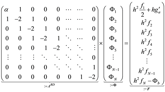
The system of linear equations associated to the Boundary Problem of type Robin-Robin can be written:
 (5)
(5)
At boundary points, the discretization of the conditions gives:
 (6)
(6)
The approximate values of the scalar field at additional imaginary points  and
and  can be eliminated. This is done considering the discrete differential equation at boundary points
  and
and , with the Equation (6). One obtains the following equation at point a
 :
:
 (7)
(7)
and the following equation at point b :
:
 (8)
(8)
One remarks that the additional points are not included in the calculations. They allowed the use of the centered difference approximation; even at the boundary points. Therefore, the truncation error behaves like  [3] .
[3] .
The vector  can be defined with its components
 :
:
 (9)
(9)
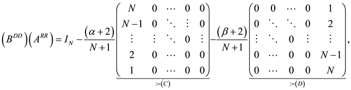
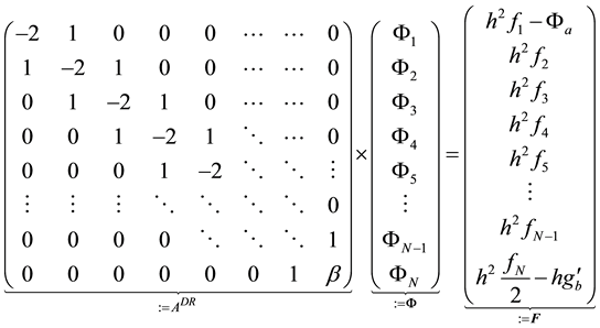
Combining the Equations (5), (7), and (8); one gets the following matrix equation:
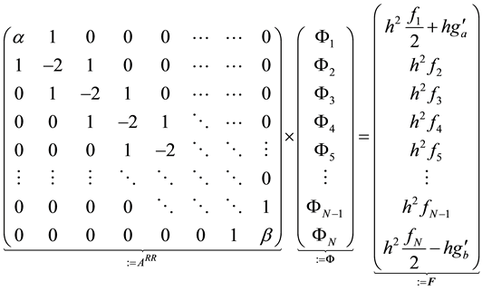 (10)
(10)
 is the discretization matrix in the case of boundary conditions of type Robin-Robin (RR). This matrix is widespread in the literature. The Equation (10) can be solved with methods such as Gaussian elimination
 , or the Thomas algorithm
  [6] .
[6] .
We propose, here, a new method of resolution, faster and more accurate than that of Thomas; as we have already done for the boundary problem of type (DD) [1] , and (ND) or (DN) [2] . This method is based essentially on the exact formulation of the inverse of the matrix . The formula of the inverse of the discretization matrix will be determined explicitly and directly. We denote it
 .
.
4. Inverse of the Matrix ARR
The matrix  is symmetric and its determinant
  depend on the coefficients
  and
and . The
. The
calculation of  permits to verify the regularity of the matrix
  i.e. its invertibility. Exploiting the re-
sults of [1] and [2] , the formula of the determinant of  can be deduced. It holds:
 (11)
(11)
This determinant is zero for the case of boundary conditions of type Neumann-Neumann (NN), which corresponds to . Apart from this case,
  is different from zero and the inverse of the matrix
  exists.
Now the inverse of the matrix  will be determined, using the matrix associated to the problem (DD), which is resolved in [1] :
 (12)
(12)
Since  and its inverse
  are known [1] , one can multiply the Equation (12) by
 , whose exact formula is known. One gets:
 (13)
(13)
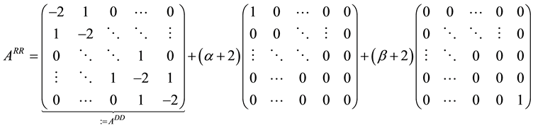
where  is the identity matrix of size N. The matrices (C) and (D) are defined in following manner, respectively:
 (14)
(14)
 (15)
(15)
The matrices (C) and (D) can be factorized and put in the form  and
and
 . One obtains, for the matrix (C):
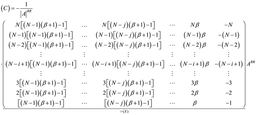 (16)
(16)
and for the matrix (D), one gets:
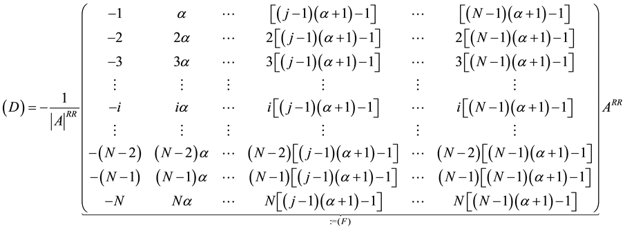 (17)
(17)
The Equation (16) shows that the matrix (E) is defined in the following manner:
 (18)
(18)
From the Equation (17), it is noted that the matrix (F) is defined in the following manner:
 (19)
(19)
Thus, the matrix Equation (13) becomes:
 (20)
(20)
And therefore, one has the relation that provides the inverse of the matrix :
:
 (21)
(21)
So, we get , inverse of the matrix
 . This famous matrix is inverted exactly and in a elegant manner [5] [7] - [10] . We gave to the matrix
  the name Bira_RR Matrix. It holds:
 (22)
(22)
with
 (23)
(23)
The Equation (22) is very important in the field of numerical resolution of differential equation in one dimension. Because it presents the exact formula of the famous matrix . It allows to solve the Equation (10) in a extremely fast way, very precisely, and independently of the RHS. It provides an innovative solution to the Poisson equation for the case of boundary conditions of type Robin-Robin.
A simple matrix-vector multiplication gives the solution of the differential equation. But we are not limiting there. Because, by exploiting the properties of the matrix , we can greatly reduce the cost in time and memory space.
A further analysis of the matrix  gives the solution
  in any mesh point
 :
:
 (24)
(24)
where :
:
 (25)
(25)
This latter equation is the same as the following [1] :
 (26)
(26)
The analysis of this solution shows that one loop is sufficient to obtain the solution  at point
 . This solution given by the Equation (24) has been obtained independently from the RHS. So it is a straightforward solution that does not use the RHS of the differential equation. In addition, a programmer does not need to declare arrays to store matrices or vectors.
This solution in Equation (24), combined with Equation (5), corresponds to an algorithmic complexity of . It is stable, robust, and very economical with respect to memory occupation.
The Equation (24) is solution for boundary problems satisfying  and
and  (RR). It is also solution of boundary problems of type Robin-Neumann (RN) or Neumann-Robin (NR).
5. Verification with a Robin-Robin (RR) Boundary Problem
We consider a scalar field , defined in [0, 1], which satisfies
 ,
,
in ]0, 1[. The field  fulfills the following Robin-Robin boundary conditions as in (27):
 (27)
(27)
where the parameters ,
,  ,
,  , and
, and  are well known real constants. The exact solution can be expressed as follows:
 (28)
(28)
of course, for .
.
The mesh is taken as specified in Figure 1: ,
, .
.
To verify our new method of resolution, we choose: ,
,  and
and . It follows:
 and
and . Also, we choose:
  and
and .
.
The computed results are shown in Table 1.
The obtained solution, with our new method, using the finite difference method, is very accurate; as Table 1 above shows. We denotes  the relative error in each point
 :
:
 (29)
(29)
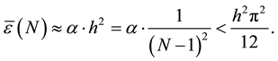
From Table 1, one can deduce the average relative error, which general expression is given as following:
 (30)
(30)
It hols: .
.
The sensibility of our new method can be determined by plotting the average relative error  for different values of N. Then, we got the curve shown in Figure 2, which is a hyperbola that can be assumed to be

Table 1. Numerical results and relative error.
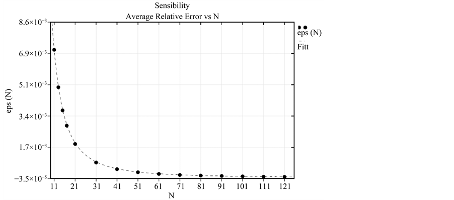
Figure 2. Sensibility for RR boundary conditions.
proportional to .
.
Thus, a curve fitting of the sensibility can be given with:
 (31)
(31)
where . The two curves are shown in Figure 2. The average relative error
  be-
be-
haves like a truncation error that can be expressed in the following manner .
.  designates
the fourth order derivative of the exact function  in a point (here C), which belongs to the interval [a, b].
Combining the given function , the exact function
 , and the results from the fitting, one gets [6] :
 (32)
(32)
So, we have demonstrated that this new method is very fast, very efficient. In addition, it is very economical in terms of occupation of memory space. It is also very accurate.
The matrix ARR is inverted analytically and in a accurate manner; independently of the RHS.
The behavior of the truncation error is very interesting as shown in the sensibility curve.
The resolution of the remaining cases Dirichlet-Robin (DR) and Robin-Dirichlet (RD) presents no difficulty. It is easy and can be done on the basis of the foregoing.
6. 1D Poisson Equation with Robin-Dirichlet and Dirichlet-Robin Boundary Conditions
6.1. 1D Poisson Equation with Dirichlet-Robin (DR) Boundary Conditions
We consider, now, a Dirichlet-Robin problem as one where the field at point a  is known and the boundary condition at point b is of type Robin:
 (33)
(33)
where . The coefficients
  and
and  are given.
For this Dirichlet-Robin boundary problem, we propose an appropriate discretization, as shown in Figure 3.
Here, the mesh points  are defined by the following relation:
 ,
, . The step
size changes and becomes: . The only imaginary point is
 . Its scalar field
  is elimi-

Figure 3. Discretization for Dirichlet-Robin boundary conditions.
nated as done in Equation (8).
Thus, considering the Equations (3)-(8) and adapting them to the (DR) problem, one gets the following matrix equation:
 (34)
(34)
One remarks that with respect to the Robin-Robin boundary problem, there is only two changes. The first component of the vector  becomes
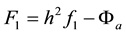 . The second one change relatively to the (RR) problem is that their matrices are related by:
 . Therefore, the inverse of the matrix
  is:
is: . Then, the solution of the Dirichlet-Robin boundary problem is known, considering the equations (22)-(26), and the change of
 , and replacing
  by
by .
.
6.2. 1D Poisson Equation with Robin-Dirichlet (RD) Boundary Conditions
We consider, now, a Robin-Dirichlet problem as one where the field at point b  is known and the boundary condition at point a is of type Robin:
 (35)
(35)
where . The coefficients
  and
and  are given.
For this (RD) boundary problem, we propose the following appropriate discretization, as shown in Figure 4.
Here, the mesh points  are defined by the following relation:
 ,
, . The
. The
step size changes and becomes: . The imaginary point is
 . Its scalar field
  is eliminated
as done in Equation (7).
Thus, considering the Equations (3)-(8) and adapting them to the (RD) problem, one gets the following matrix equation:
 (36)
(36)
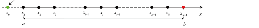
Figure 4. Discretization for Robin-Dirichlet boundary conditions.
One remarks that with respect to the Robin-Robin boundary problem, there is only two changes. The last component of the vector F becomes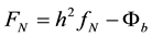 . The second one relatively to the (RR) problem is that the matrices of the two problems are related by:
 . Therefore, the inverse of the matrix
  is:
is: . Then, the solution of the Robin-Dirichlet boundary problem is known, considering the Equations (22)-(26), and the change of
 , and replacing
  by
by .
.
7. Conclusion
This study relates to the resolution of 1D Poisson equation, with the general case of Robin boundary conditions. The major innovation that is presented, is the exact formulation of the inverse of the discretization matrix, which is obtained from using the finite difference method. This remarkable and direct inversion of this matrix provides an elegant and efficient solution to this very important differential equation. This new proposed method of resolution is precise, economic in memory occupancy, and extremely fast. It can serve as reference for solving numerically the 1D Poisson equation and the stationary wave or heat equation.
References
- Gueye, S.B. (2014) The Exact Formulation of the Inverse of the Tridiagonal Matrix for Solving the 1D Poisson Equation with the Finite Difference Method. Journal of Electromagnetic Analysis and Applications, 6, 303-308. http://dx.doi.org/10.4236/jemaa.2014.610030
- Gueye, S.B., Talla, K. and Mbow, C. (2014) Solution of 1D Poisson Equation with Neumann-Dirichlet and Dirichlet-Neumann Boundary Conditions, Using the Finite Difference Method. Journal of Electromagnetic Analysis and Applications, 6, 309-318. http://dx.doi.org/10.4236/jemaa.2014.610031
- Kreiss, H.O. (1972) Difference Approximations for Boundary and Eigenvalue Problems for Ordinary Differential Equations. Mathematics of Computation, 26, 605-624. http://dx.doi.org/10.1090/S0025-5718-1972-0373296-3
- Engeln-Muellges, G. and Reutter, F. (1991) Formelsammlung zur Numerischen Mathematik mit QuickBasic-Program- men, Dritte Auflage. BI-Wissenchaftsverlag, Mannheim, 472-481.
- LeVeque, R.J. (2007) Finite Difference Method for Ordinary and Partial Differential Equations, Steady State and Time Dependent Problems, SIAM, 15-25. http://dx.doi.org/10.1137/1.9780898717839
- Conte, S.D. and de Boor, C. (1981) Elementary Numerical Analysis: An Algorithmic Approach. 3rd Edition, McGraw- Hill, 153-157.
- Mathews, J.H. and Fink, K.K. (2004) Numerical Methods Using Matlab. 4th Edition, Prentice-Hall Inc., New Jersey, 323-325, 339-342.
- Sadiku Matthew, N.O. (2000) Numerical Techniques in Electromagnetics. 2nd Edition, CRC Press, Boca Raton, 610-626. http://dx.doi.org/10.1201/9781420058277
- Gustafson, K. (1988) Domain Decomposition, Operator Trigonometry, Robin Condition. Contemporary Mathematics, 218, 432-437. http://dx.doi.org/10.1090/conm/218/3039
- Reinhold, P. (2008) Analysis of Electromagnetic Fields and Waves: The Method of Lines. John Wiley, Chichester, 9.