Journal of Electromagnetic Analysis and Applications
Vol.4 No.5(2012), Article ID:19522,7 pages DOI:10.4236/jemaa.2012.45026
Simulation of Modes of Ionosphere Alfvén Resonator with High Quality Factors in the Case of Oblique Geomagnetic Field
![]()
1Autonomous University of State Morelos (UAEM), CIICAp, Morelos, Mexico; 2Center of Geoscience, Autonomous National University of Mexico (UNAM), Queretaro, Mexico.
Email: *svetlana@uaem.mx, v_grim@yahoo.com
Received March 16th, 2012; revised April 13th, 2012; accepted April 23rd, 2012
Keywords: Alfvén Resonator; Resonant Modes; Quality Factors; Modulation
ABSTRACT
The properties of the ionosphere Alfvén resonator (IAR) in the general case of an oblique geomagnetic field are investigated. The modes at the frequencies f = 0.2 - 10 Hz well localized within the ionosphere are considered, which are important for the lithosphere—ionosphere coupling. An attention is paid to the modes with quite high quality factors , where
 . A proper selection of calculated eigenfrequencies has been realized. Two independent simulation algorithms have been proposed. The resonant frequencies and the profiles of magnetic field components of the modes have been calculated. The modulation of electron and ion concentrations at the heights 170 - 230 km leads to essential shifting the resonant frequencies.
1. Introduction
The ionosphere creates for the Alfvén waves some resonator, which is called as the ionosphere Alfvén resonator (IAR), in the frequency range f = 0.05 - 10 Hz [1-4]. The resonant modes are localized in the vertical direction within the ionosphere F-layer, the heights 150 - 400 km with the maximum values of the electron concentration, and bounded by the gyrotropic E-layer from below and the magnetosphere from above [5-10]. Because the ionosphere is an open system, the magnetic field of IAR can reach the Earth’s surface and can penetrate into the lithosphere.
The simplest model of IAR considers the vertical direction of the geomagnetic field along OZ axis and permits to get the analytical results [10]. In the ionosphere F-layer the gyrotropy is neglected (g » 0), and an inequality is valid: , where the tensor of effective permittivity is:
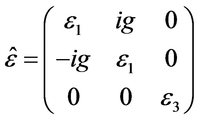
A dependence of e1(z) is taken into account. In the ionosphere E-layer the gyrotropy is essential, and the impedance boundary condition is introduced at z » 120 km. Nevertheless, the simplified approach cannot be used in the case of the oblique geomagnetic field. Moreover, in the F-layer at the heights z ~ 150 - 200 km the gyrotropy is not zero, and its influence on the resonances is essential. Also, generally speaking, the magnetic field of IAR penetrates down to the Earth’s surface and can be measured there. Therefore, a more exact theory should be put forward. At the same time, the theory should not be cumbersome, because the interpretation of the results must be clear.
As usually, natural resonances in geophysics possess relatively low quality factors [10]. But in the open systems resonances of low quality factors do not have any physical sense and cannot be released separately, because of the presence of continuum spectrum. Therefore, some selection of the formally calculated resonance modes should be realized. The modes possessing higher quality factors can be useful for detecting the lithosphere— ionosphere coupling. Namely, these modes can be modulated by the acoustic gravity waves and internal gravity waves of ULF range that are excited at the Earth’s surface, move upwards and reach the ionosphere.
The propagating modes in the ionosphere waveguide were considered in the papers [11-13]. The dependencies of the complex wave numbers on the real frequency were investigated within the waveguide, which was assumed uniform in the horizontal plane of propagation. In the resonator problem, considered in the present paper, the complex eigenfrequencies with relatively small imaginary parts should be investigated. Whereas in [11-13] the vertical profiles of the waveguide modes were not presented, the vertical profiles of the modes of the resonator are of special interest.
In the present paper the resonant modes of IAR are calculated in the case of arbitrary direction of the geomagnetic field. The selection of the modes has been done. Namely, the selected modes possess quite high quality factors 5 - 20. Also they are well localized within the ionosphere, have a weak dependence on inclination of the geomagnetic field and are separated from each other. There are several modes occur that satisfy the pointed above demands. The modulation of the electron concentration at the heights 170 - 230 km can shift the resonant frequencies; it is important for the lithosphere—ionosphere coupling.
2. Basic Equations
Consider a model for EM oscillations of ULF-ELF ranges f = 0.2 - 10 Hz localized in the ionosphere. The modes at frequencies f = 0.005 - 0.1 Hz [14-17] are not considered here, because they penetrate highly into the magnetosphere and possess low quality factors.
The EM field of resonances can penetrate into the atmosphere, lithosphere, and the magnetosphere. Therefore, the coordinate z changes within the limits –Le < z < Lz, where Le = 30 km, i.e. the thickness of the lithosphere, Lz = 800 km within the magnetosphere. A general case of an oblique geomagnetic field is investigated; the inclination angle of the geomagnetic field H0 is Q.
The system is assumed as uniform in (XY) plane. The curvature of the Earth’s surface is neglected, because the condition  is valid. Basic volume equations are [10,11,18]:
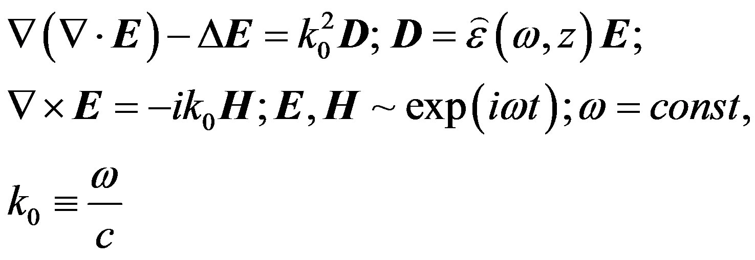 (1)
(1)
Here w is the frequency of resonance oscillations, it is generally complex: w = w′ + iw″ (w″ > 0, because of losses). Such losses are due to both the non-Hermitian part of the effective permittivity tensor, i.e. the dissipation, and the leakage of the EM field into the magnetosphere. Our goal is to calculate the set of possible eigenfrequencies and profiles of the modes of the IAR in the pointed above frequency interval.
Generally for magnetosphere and ionosphere, the expression for the effective permittivity tensor  is [10,18]:
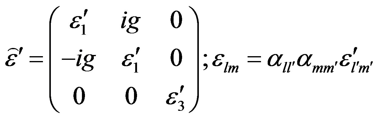
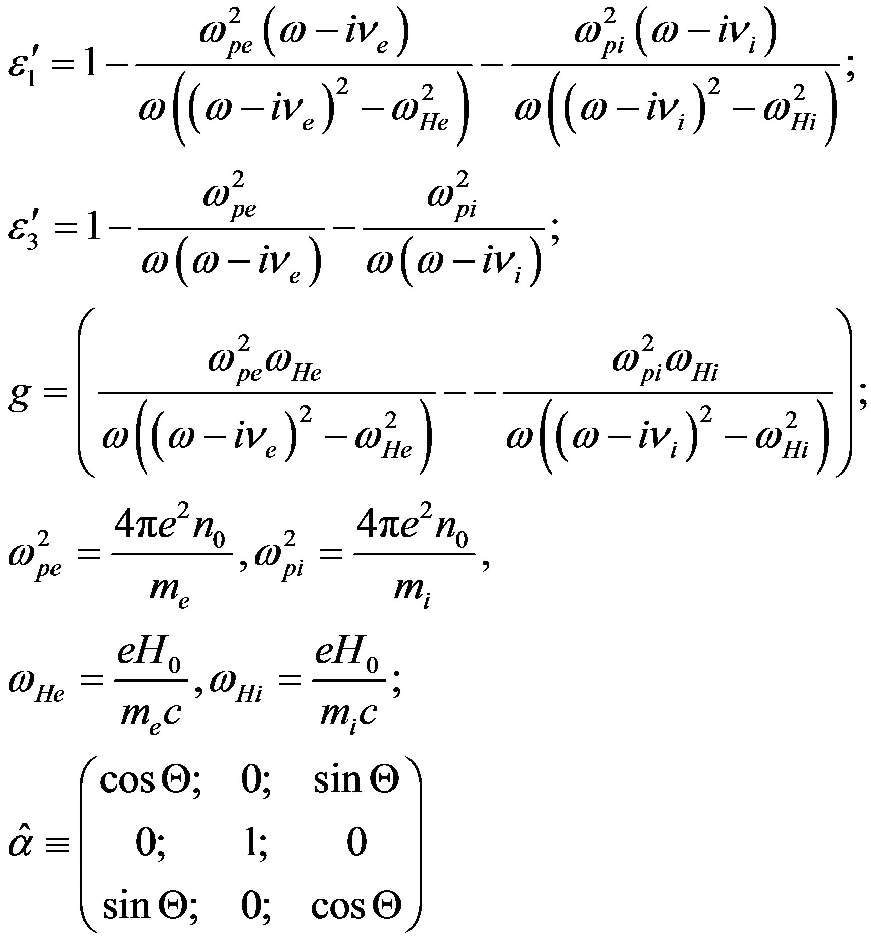 (2)
(2)
Here αll´ are the elements of the matrix  of rotation from
  frame to (XYZ) one. The axis OZ′ is directed along the geomagnetic field H0, the axis OZ is directed vertically upwards. The absolute system of units is used here.
The lithosphere is considered as a medium with finite conductivity s [10], which depends on the coordinate z:
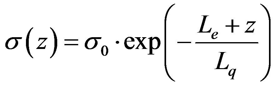
The effective dielectric permittivity is: 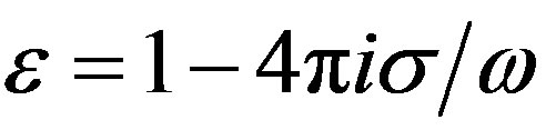 there. The value of s0 has been chosen as
  in absolute units. For the chosen frequency range
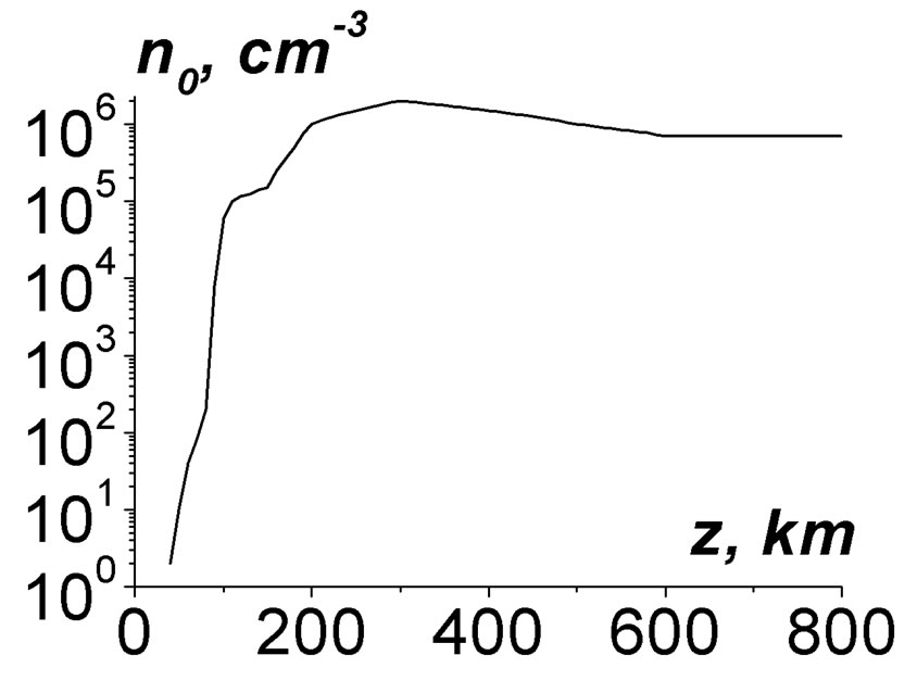
  Hz the properties of resonant modes depend weakly of the parameters s0 and Lq. At lower frequencies f < 0.1 Hz this dependence can be more essential. The parameters of the ionosphere and the magnetosphere used in simulations are given in Figure 1.
Generally, EM field depends on all coordinates x, y, z. But, because the scale of the system along OZ axis is of about 10 - 30 km, whereas the scale in the horizontal plane (x,y) is  km, it is possible to consider the oscillations that depend on the coordinate z only.
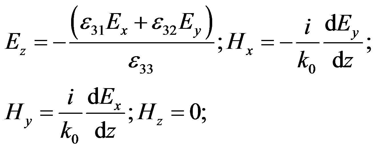
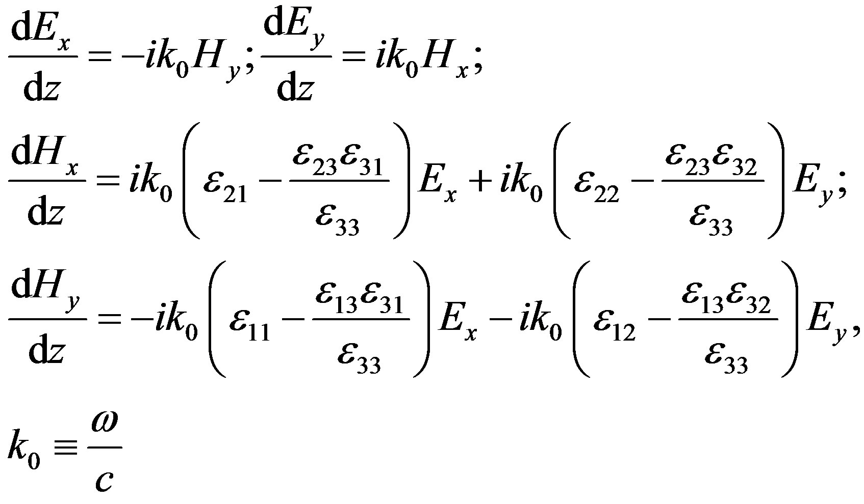
From Equation (1) one can derive the equations for Ex, Ey components [18]:
 (a)
(a)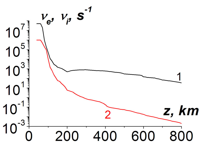 (b)
(b)
Figure 1. Dependence of electron concentration (a) and collision frequencies of electrons (curve 1) and ions (2) (b) on heights z.
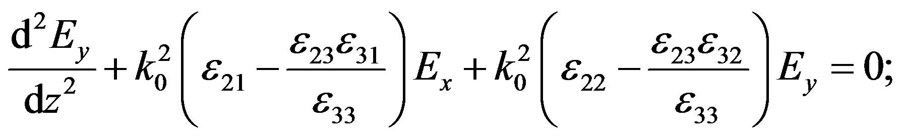 (3)
(3)
Equations (3) should be added by boundary conditions. In the deep lithosphere ( ), it is possible to put Ex,y = 0. In the magnetosphere, only outgoing waves exist, i.e. the radiation condition is valid. These waves are the Alfvén wave of Ex polarization and the fast magnetosonic one of Ey polarization [10,18]. Therefore, the boundary condition at z = Lz can be presented in the following way:
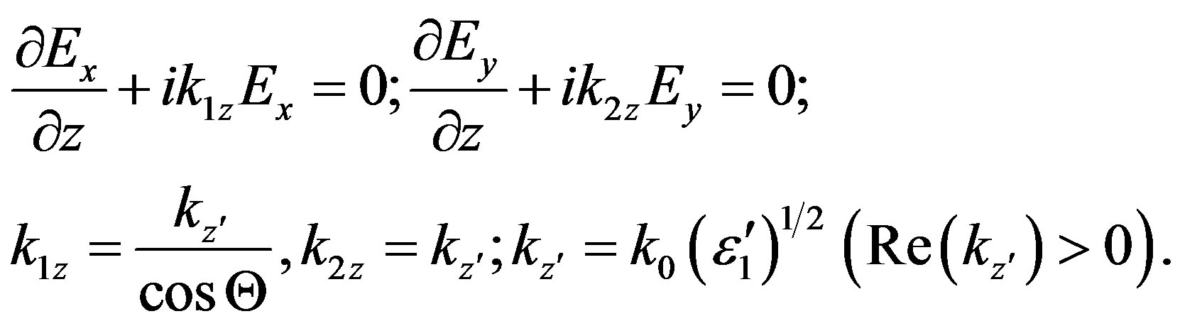 (4)
(4)
Here k1z and k2z are the wave numbers of the waves pointed above [10]. The inequality  has been used there. Note that from the side of the magnetosphere IAR is an open structure. Therefore, its modes are generally leaky, and
  [19].
[19].
Thus, the modes of IAR are nonzero solutions of uniform Equations (3) added by uniform boundary conditions.
3. Method of Simulations
The Equations (3) with the boundary conditions (4) have been approximated by finite differences:
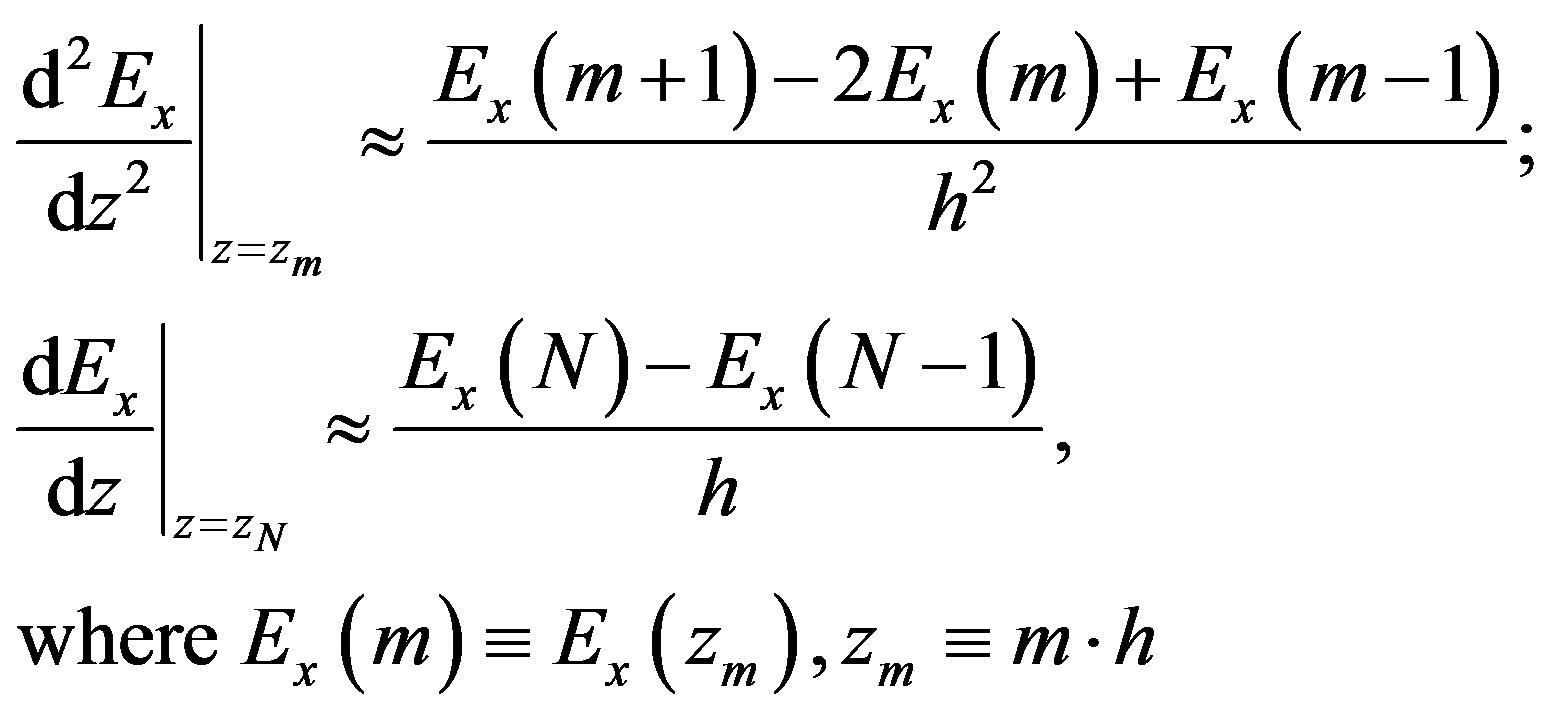 (5)
(5)
Here h is the step along OZ axis; Lz = N×h, Le = Ne×h.
As a result, a set of uniform linear equations has been formed. They possess a matrix structure:
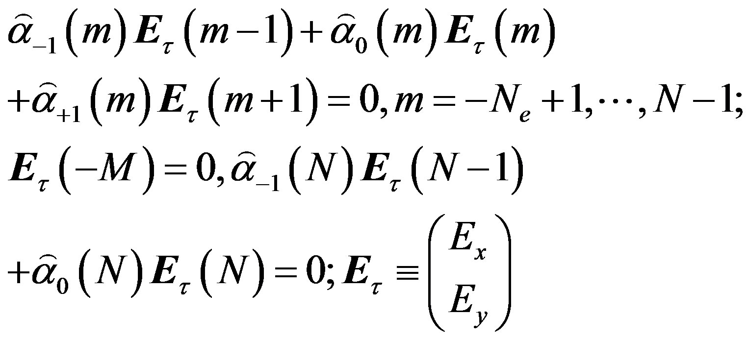 (6)
(6)
Here  etc. are matrices 2 ´ 2. This set of equations has been solved by the factorization method. Namely, it is possible to represent:
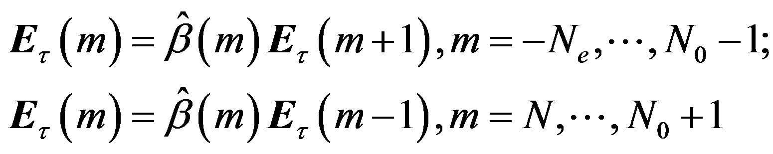 (7)
(7)
and to calculate the matrices  consecutively, step by step. The point z = L0 º N0×h is within the ionosphere F-layer, L0 = 200 - 300 km. As a result, at m = N0 it is possible to get a single matrix equation for Et(N0) as:
 (8)
(8)
Nontrivial solutions are searched: Et(N0) ¹ 0. Therefore, the following determinant is equal to zero:
 (9)
(9)
This is the dispersion equation for the set of complex eigenfrequencies ωj, j = 1,2,··· The eigenfrequencies depend neither on the choice of the spatial step h nor on the position of the point z = L0.
To solve the dispersion equation, the following iteration procedure has been applied. The equation under solution is: . The following representation has been used:
 , where s is the number of iteration. Within the parabolic approximation, it is possible to write down:
 ; this is a quadratic equation for
 . The minimum root has been taken the iteration. The realization of this procedure is not difficult, because the solutions with relatively small imaginary values and, correspondingly, quite high quality factors are searched. Therefore, the initial approximation for each eigenfrequency has been chosen as real. The derivatives
  have been computed by finite differences by means of the five point scheme. A simpler linear approximation, i.e. the Newton method, also has been applied, but the quadratic approximation has demonstrated a faster convergence.
To check the obtained results, another method to solve the problem has been proposed, which is similar to [20]. It is possible rewrite Equations (2) like a set of equations of the first order for Ex, Ey, Hx, Hy [11]:
 (10)
(10)
In the matrix form, this set of equations is:
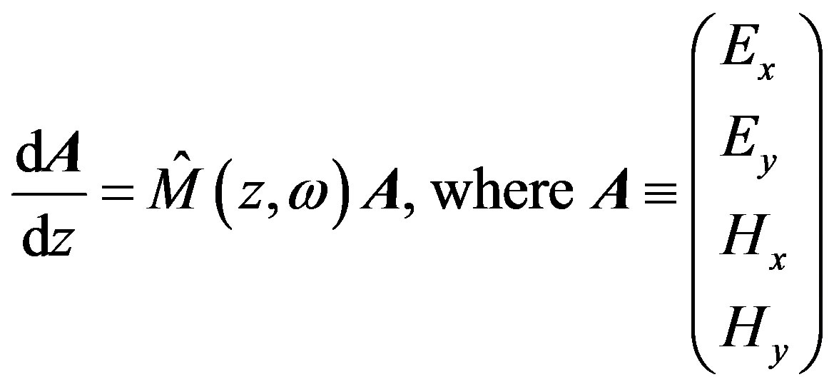 (11)
(11)
The boundary conditions at z = Lz also been presented for Ex, Hy, Ey, Hx:
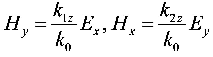 (12)
(12)
Here k1z, k2z have been determined in Equation (4).
Then the solutions of the set differential equations can be represented symbolically as [21]:
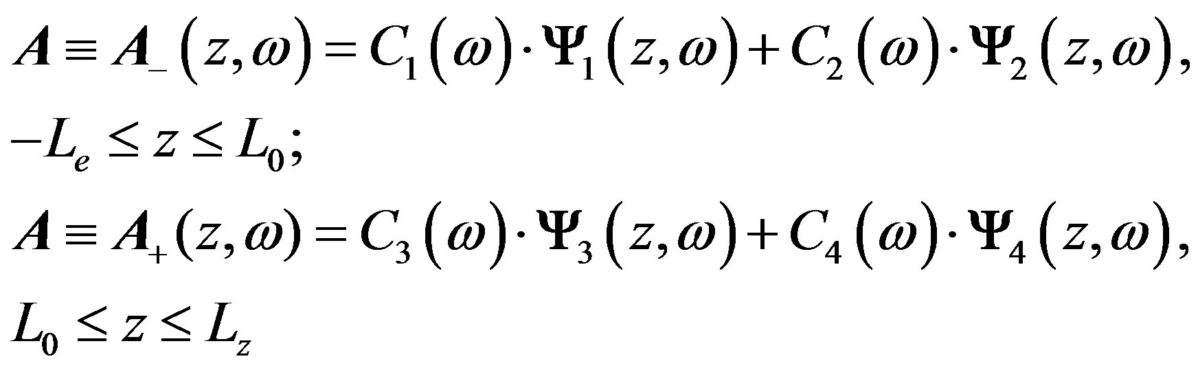 (13)
(13)
Here  are linearly independent partial solutions of differential equation that satisfy the boundary conditions at z = –Le;
  are ones that satisfy the boundary conditions at z = Lz.
It is easy to compute the proper partial independent solutions in the following manner. At z = –Le, lithosphere, the boundary conditions for  and
and  are: Ex = Ey = Hy = 0, Hx = 1 and Ex = Ey = Hx = 0, Hy = 1, correspondingly. At z = Lz, magnetosphere, the boundary conditions for
  and
and  are: Ex = 1, Ey = Hx = 0,
  and Ex = Hx = 0, Ey = 1,
  , correspondingly. Knowing the proper boundary conditions, one can solve the set of linear ordinary differential equations (11) by standard numerical methods. We have used the implicit Adams method, because of its good stability [21] and accuracy.
The point z = L0 is an arbitrary point within the ionosphere F-layer: L0 = 200 - 300 km. It can be the same or different as considered in the first method. From continuity of the solution:  one can obtain the set of four linear uniform equations for coefficients C1,2,3,4. Because these coefficients cannot be zeros simultaneously for a non-trivial solution, the equating of the determinant of this set to zero yields the equation for eigenfrequencies. This equation has been solved by the same iteration procedure as for the first method.
4. Results of Simulations
The following parameters have been used in simulations: the depth of the lithosphere is Le = 30 km, the upper limit in the magnetosphere is Lz = 800 km, the scale of changing the lithosphere conductivity is Lq = 5 km. The results of simulations are tolerant to a possible change of the pointed above parameters (Le, Lz, Lq), of the position of the central point z = L0, and of the spatial step h, when h ≤ 1 km. The eigenfrequencies obtained by two pointed above methods have coincided. The validity of obtained eigenfrequencies and solutions for the field components has been checked directly by means of substitution to Equations (3) and Equations (10). Maximum relative error has been smaller than 10–6. Typically the number of the discretization points is N = 2000 … 20000.
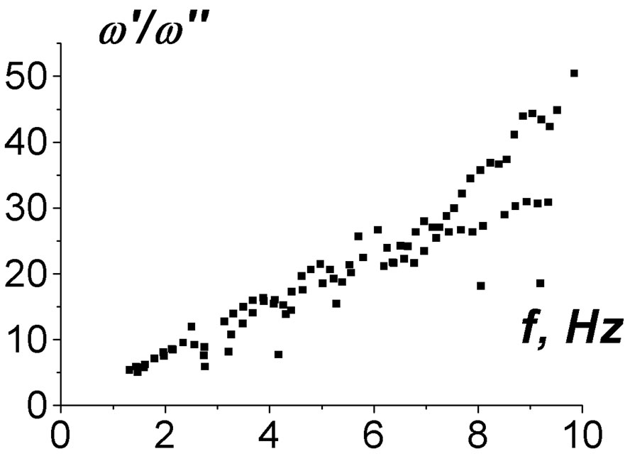
The sets of resonant frequencies of IAR formally calculated as a solution of uniform differential equations added by uniform boundary conditions are given in Figure 2 for different inclination angles of the geomagnetic field (Q = 0, 30˚, 60˚).
Only the eigenfrequencies with enough high values of a quality factor are presented. Namely, the ratio between the real part of angular eigenfrequency  and its imaginary part
  should be
  (w = 2pf, where f is
 (a)
(a)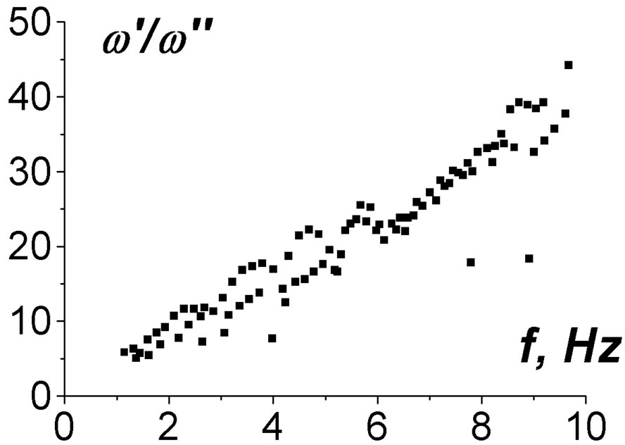 (b)
(b)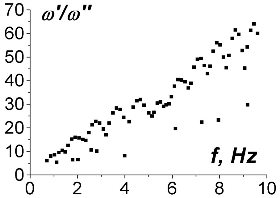 (c)
(c)
Figure 2. Formally calculated eigenfrequencies of IAR before selection. Here w′/w″ are quality factors. Part (a) is for Q = 0; (b) is for Q = 30˚; (c) is for Q = 60˚.
the ordinary frequency). For the modes at lower frequencies f < 0.2 Hz, which penetrate highly into the magnetosphere z > 800 km, the computed quality factors [11,12] are lower: . In that case there exists the principal problem of the difference of free oscillation modes, where the values of
  are taken at the complex values of w, and the “loaded”, or excited by external currents, modes with
  [19]. Moreover, for open systems the modes with low quality factors do not have any physical sense, because the energy of electromagnetic field of continuum spectrum is comparable with the discrete modes [19].
One can see that there are a lot of computed eigenfrequencies. But only a few solutions can be associated with true modes of IAR, which can be observed experimentally. A proper selection of the true modes should be realized after this primary computing.
The following conditions it is necessary to use for the modes: 1) a good localization within the ionosphere, i.e. the weak leakage; 2) a weak dependence on inclination of the geomagnetic field; 3) each eigenfrequency should be well separated from other ones.
The first condition is important because the IAR is an open system and the modes principally leak into the magnetosphere. Because within the ionosphere and magnetosphere the energy is concentrated in the magnetic field components, the true modes should possess the values of the magnetic fields at the heights z ~ 600 km no more than 20% that the maximum ones within the ionosphere F-layer (z = 200 - 300 km). Otherwise, the modes cannot be excited separately from the continuum spectrum.
The second condition is due to the dependence of electromagnetic properties of the ionosphere and magnetosphere on the inclination of the geomagnetic field. In the case when horizontal distance changes on 500 km, the inclination angle Q of the geomagnetic field changes on »5˚. Under this change of the angle Q the real part of the resonant frequency should be displaced no more than on the value of its imaginary part.
The third condition is taken into account, because the phenomenon of overlapping resonances is not considered. The eigenfrequencies, which are separated at the distances smaller than their imaginary parts, have been eliminated. This condition is not so rigorous as previous ones; nevertheless, we do not consider overlapping the resonances here.
In Figure 3 dependences of the selected eigenfrequencies on the inclination angle Q are presented. In Figures 4, 5 the profiles of all the selected modes are given. One can see that the magnetic field components are localized in the ionosphere F-layer. The quality factors are of about ; thus, these modes can be excited
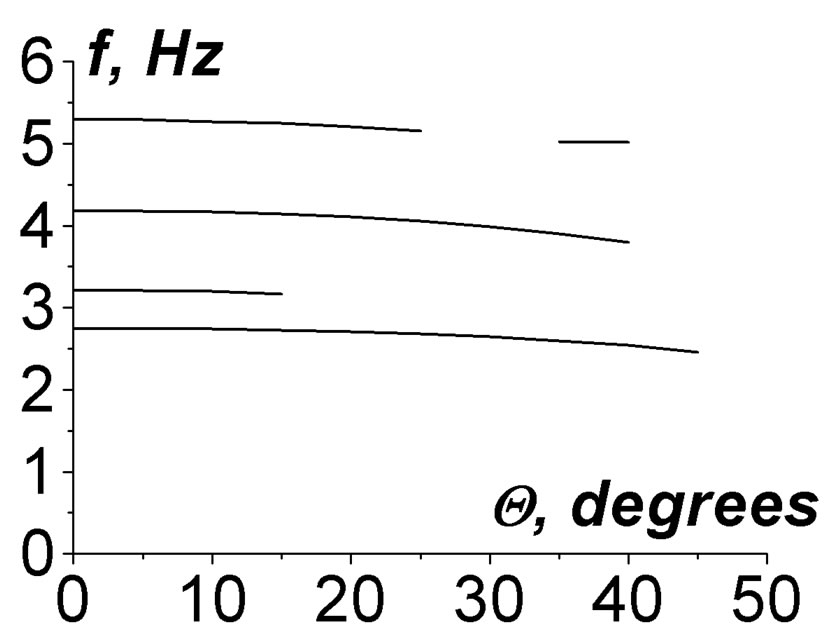
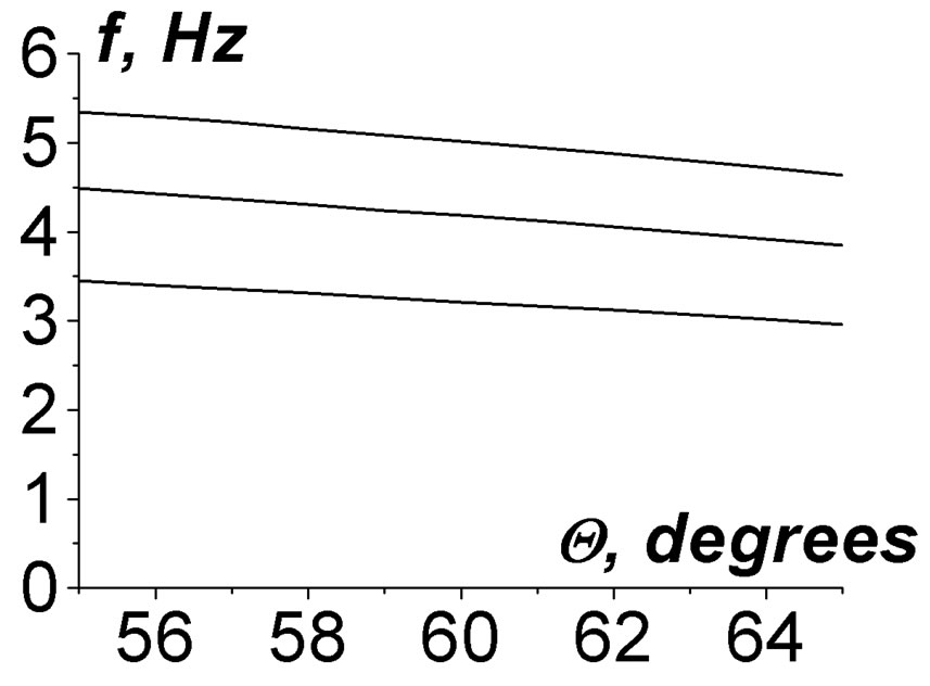
Figure 3. Dependence of frequencies of selected (true) resonant frequencies IAR on the inclination angle of the geomagnetic field.
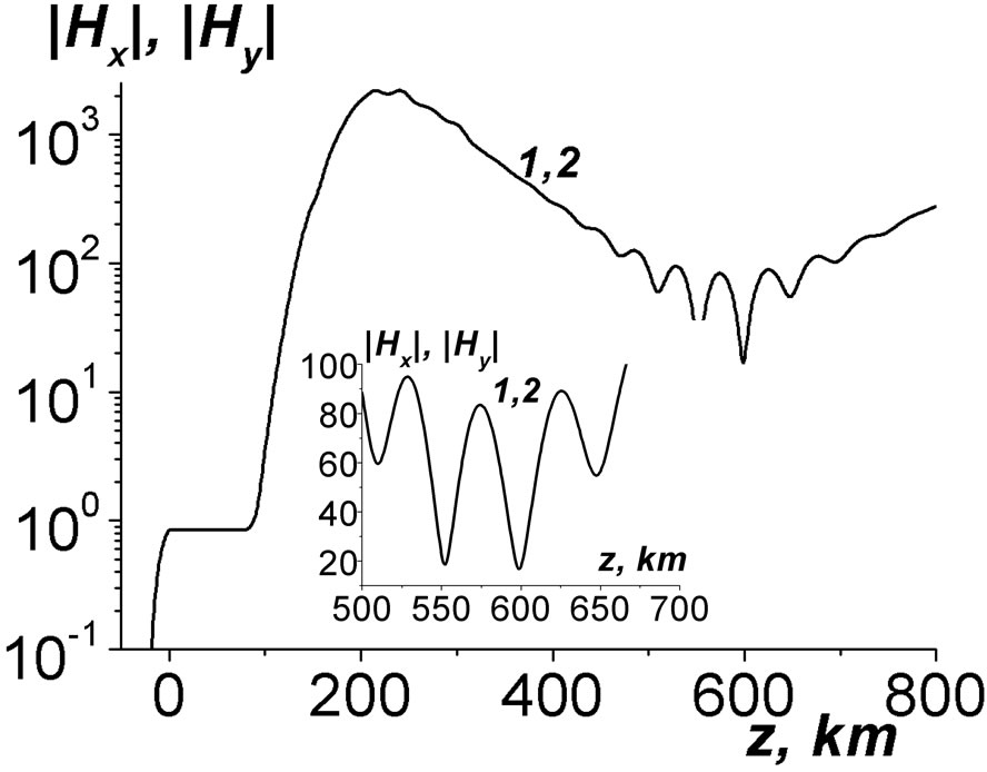
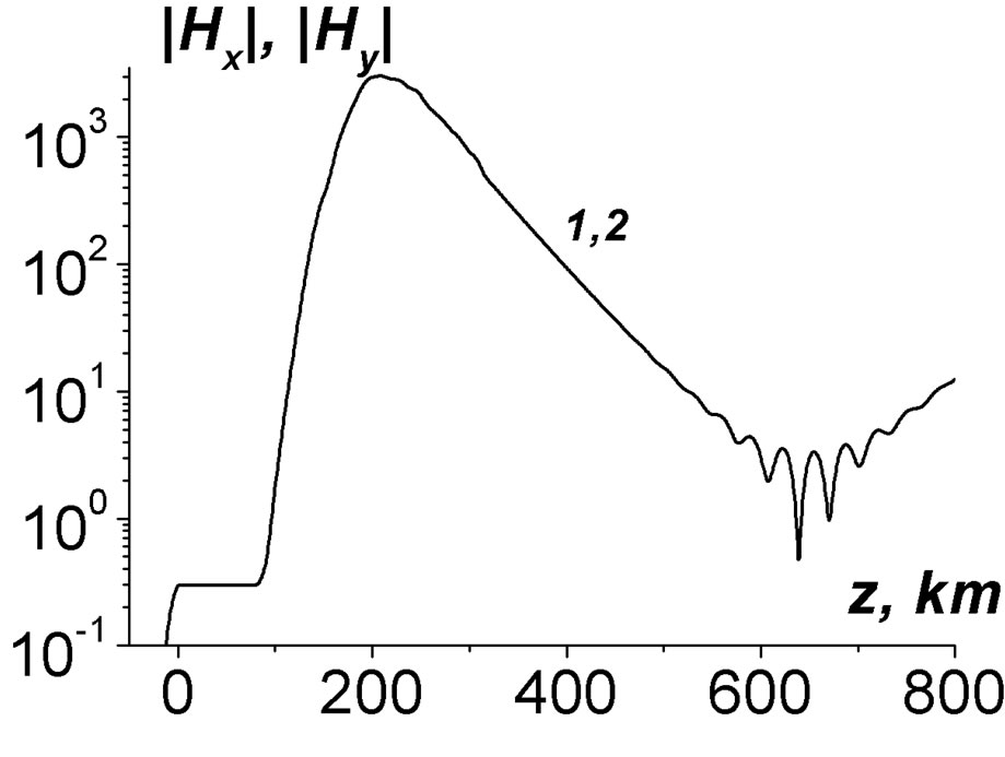
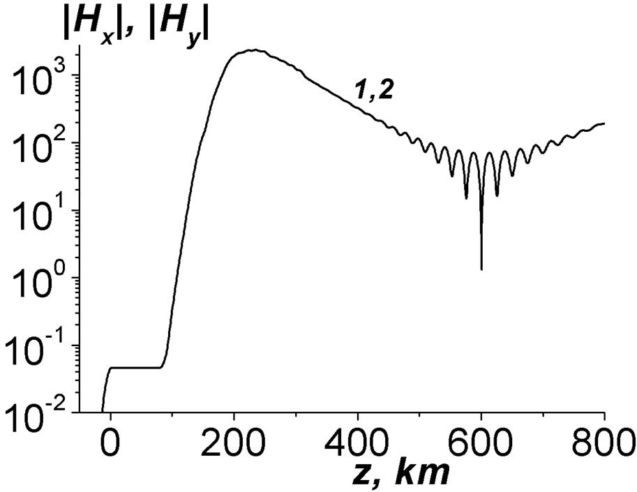
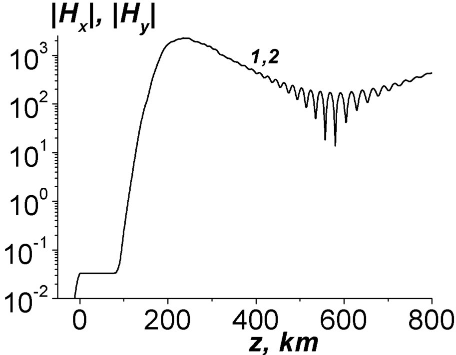
Figure 4. The true mode profiles at the inclination angle Q = 0. Curve 1 is |Hx(z)|, 2 is |Hy(z)| (at zero angle they coincide).
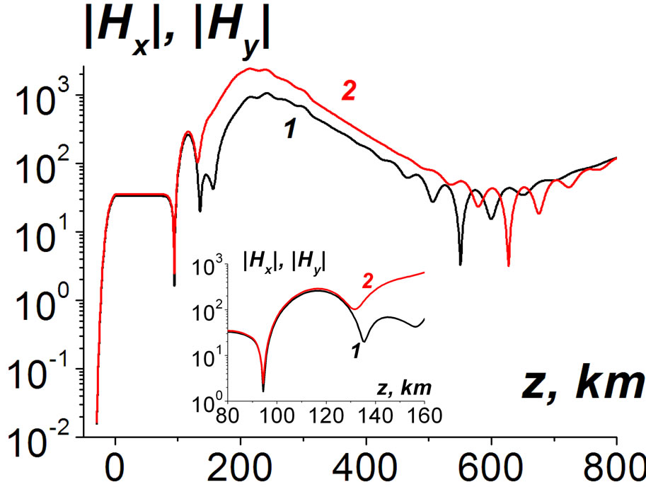
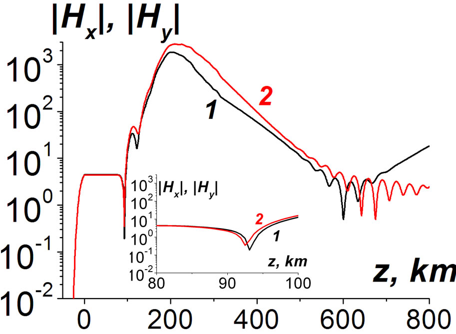
Figure 5. The true mode profiles at Q = 30˚. Curve 1 is |Hx(z)|, 2 is |Hy(z)|.
effectively by ionosphere current sources or by external excitation by Alfvén wave beams from the magnetosphere.
The profiles of the modes possess the oscillatory character near the minimum values of the EM field. These oscillations can be explained in the following manner. At the periphery z ~ 600 km the EM field includes both the outgoing wave and reflected one. The reflected wave is small and it appears due to the inhomogeneities of the upper ionosphere. But near the minimum also the outgoing wave is small, too. Therefore, the interference of the outgoing wave and the reflected one takes place, see the insert in Figure 4. This interference manifests near the minimum point only. Analogous oscillations of smaller values occur also in the lower ionosphere, z » 100 km, where strong gradients of the electron concentrations are available, see inserts in Figure 5. In Equations (3) for Ex, Ey the derivatives from  are absent. Therefore, there is no problem with the realization of numerical algorithms, when the spatial step h ≤ 0.1 km is much smaller than the spatial scale of change of the electron concentration ~ 5 km there.
Because the resonance modes possess quite high quality factors, they are sensitive to an influence of the lithosphere—ionosphere coupling. Such a coupling can be realized by the acoustic-gravity waves (AGW) and internal gravity ones (IGW) of ULF range. These waves can be excited by the sources on the Earth’s surface and reach the ionosphere E and F layers [22]. Because the mass density of the ionosphere is much more low that the near-Earth atmosphere, the amplitudes of the oscillations of the particles can be high. The penetration of AGW and IGW leads to the modulation of electron concentration within the ionosphere. In our simulations a possible modulation of electron (and ion) concentration n has been taken into account as:
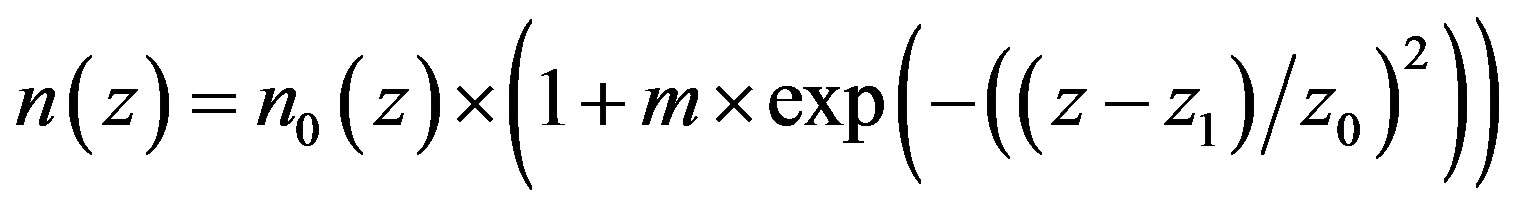
The maximum influence of modulation of the electron concentration on IAR eigenfrequencies occurs, when z1 = 170 ··· 230 km, as our simulations have shown.
This modulation shifts the eigenfrequencies of IAR. Moreover, as our calculations have demonstrated, some resonances can be removed completely. In Figure 6 a dependence of eigenfrequencies on the modulation m is presented. In simulations, the values z1 = 200 km, z0 = 30 km have been used.
A possible modulation can be influenced by AGW or IGW. AGW at the frequencies W ~ 0.05 s–1 when moving upwards can reach the heights z ~ 150 - 300 km [23]. AGW can be excited near the Earth’s surface due to seismic sources. The wave numbers of AGW are K » W/s ~ 0.1 km–1, where s » 0.5 km/s is the sound velocity. The modulation scale due to AGW is . Note that for m < –0.2 the first resonant frequency disappears due to delocalization, whereas the second resonant frequency changes its value only. The quality factors
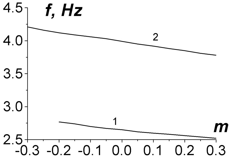
Figure 6. Possible modulation of resonant frequencies of IAR due to AGW and IGW at Q = 30˚.
 change weakly. This confirms an influence of the lithosphere—ionosphere coupling on IAR.
5. Conclusions
The resonant frequencies, quality factors, and the profiles of magnetic field components of the ionosphere Alfvén resonator modes have been calculated. A general case of an oblique geomagnetic field has been considered. It has been demonstrated that even under the inclined geomagnetic field several modes exist that satisfy the conditions of a good localization, a weak dependence on the inclination of the geomagnetic field, and separability from another possible resonance oscillations. The calculated resonant frequencies are within the frequency range f = 1 - 6 Hz. The quality factors  are of about 5 - 20, where
 . Therefore, the calculated quality factors are comparable with those for the Schumann resonances in the gap “Earth—ionosphere” and are quite high for geophysics.
The resonant frequencies can be modulated by acoustic gravity waves (AGW) and internal gravity waves (IGW) of ULF range, which are excited by lithosphere sources, move upwards, and reach the ionosphere F-layer. AGW and IGW can modulate the electron concentration of the ionosphere F-layer at heights z » 200 km, this leads to modification of parameters of IAR.
6. Acknowledgements
Authors thank SEP-CONACyT for the support of our work.
REFERENCES
- S. V. Polyakov, “On Properties of an Ionospheric Alfvén Resonator,” Symposium KAPG on Solar-Terrestrial Physics, Vol. III, Nauka, Moscow, 1976, pp. 72-73.
- S. V. Polyakov and V. O. Rapoport, “Ionospheric Alfvén Resonator,” Geomagnetism and Aeronomy, Vol. 21, 1981, pp. 610-614.
- R. L. Lysak, “Generalized Model of the Ionospheric Alfvén Resonator,” In: R. L. Lysak, Ed., Auroral Plasma Dynamics, Geophysical Monograph 80, American Geophysical Union, Washington DC, 1993, pp. 121-128. doi:10.1029/GM080p0121
- P. P. Belyaev, S. V. Polyakov, V. O. Rapoport and V. Y. Trakhtengerts, “The Fine Structure of the Radiation of an Alfvén Maser,” Geomagnetism and Aeronomy, Vol. 24, 1984, pp. 202-205.
- P. P. Belyaev, S. V. Polyakov, V. O. Rapoport and V. Y. Trakhtengerts, “Experimental Studies of the Spectral Resonance Structure of the Atmospheric Electromagnetic Noise Background within the Range of Short-Period Geomagnetic Pulsations,” Izvestiya VUZ, Radiophizika, Vol. 32, 1989, pp. 663-672.
- P. P. Belyaev, S. V. Polyakov, V. O. Rapoport and V. Y. Trakhtengerts, “The Ionospheric Alfvén Resonator,” Journal of Atmospheric—Terrestrial Physics, Vol. 52, No. 9, 1990, pp. 781-788. doi:10.1016/0021-9169(90)90010-K
- T. Bösinger, C. Haldoupis, P. P. Belyaev, M. N. Yakunin, N. V. Semenova, A. G. Demekhov and V. Angelopoulos, “Spectral Properties of the Ionospheric Alfvén Resonator Observed at a Low-Latitude Station (L = 1.3),” Journal of Geophysical Research, Vol. 107, No. A10, 2002, pp. 1281-1289. doi:10.1029/2001JA005076
- P. P. Belyaev, T. Bosinger, S. V. Isaev, V. Y. Trakhtengerts and J. Kangas, “First Evidence at High Latitudes for Ionospheric Alfvén Resonator,” Journal of Geophysical Research, Vol. 104, No. A3, 1999, pp. 4305-4317. doi:10.1029/1998JA900062
- A. G. Yahnin, N. V. Semenova, A. A. Ostapenko, J. Kangas, J. Manninen and T. Turunen, “Morphology of the Spectral Resonance Structure of the Electromagnetic Background Noise in the Range of 0.1 - 4 Hz at L = 5.2,” Annales Geophysicae, Vol. 21, No. 3, 2003, pp. 779-786. doi:10.5194/angeo-21-779-2003
- A. V. Guglielmi and O. A. Pokhotelov, “Geoelectromagnetic Waves,” IOP Publ., Bristol, 1996.
- C. Greifinger and P. S. Greifinger, “Theory of Hydromagnetic Propagation in the Ionospheric Waveguide,” Journal of Geophysical Research, Vol. 73, No. 23, 1968, pp. 7473-7490. doi:10.1029/JA073i023p07473
- P. Greifinger, “Ionospheric Propagation of Oblique Hydromagnetic Plane Waves at Micropulsation Frequencies,” Journal of Geophysical Research, Vol. 77, No. 13, 1972, pp. 2377-2391. doi:10.1029/JA077i013p02377
- C. Greifinger and P. Greifinger, “Wave Guide Propagation of Micropulsations Out of the Plane of the Geomagnetic Meridian,” Journal of Geophysical Research, Vol. 78, No. 22, 1973, pp. 4611-4618. doi:10.1029/JA078i022p04611
- M. D. Sciffer, C. L. Waters and F. W. Menk, “Propagation of ULF Waves through the Ionosphere: Inductive Effect for Oblique Magnetic Fields,” Annales Geophysicae, Vol. 22, No. 4, 2004, pp. 1155-1169. doi:10.5194/angeo-22-1155-2004
- M. D. Sciffer, C. L. Waters and F. W. Menk, “A Numerical Model to Investigate the Polarisation Azimuth of ULF Waves through an Ionosphere with Oblique Magnetic Fields,” Annales Geophysicae, Vol. 23, No. 11, 2005, pp. 3457-3471. doi:10.5194/angeo-23-3457-2005
- C. L. Waters and S. P. Cox, “ULF Wave Effects on High Frequency Signal Propagation through the Ionosphere,” Annales Geophysicae, Vol. 27, No. 7, 2009, pp. 2779- 2788. doi:10.5194/angeo-27-2779-2009
- R. L. Lysak and Y. Song, “A Three-Dimensional Model of the Propagation of Alfven Waves through the Auroral Ionosphere: First Result,” Advances in Space Research, Vol. 28, No. 5, 2001, pp. 813-822. doi:10.1016/S0273-1177(01)00508-7
- L. S. Alperovich and E. N. Fedorov, “Hydromagnetic Waves in the Magnetosphere and the Ionosphere,” Springer, New York, 2008.
- L. A. Vainshtein, “Open Resonators and Open Waveguides,” Golem Press, Boulder, CO, 1969.
- K. G. Budden, “Radio Waves in the Ionosphere,” CUP, Cambridge, 1961, pp. 493-500.
- V. A. Ilyina and P. K. Silaev, “Numerical Methods for Physicists,” Vol. 2, Institute for Computer Investigations Publ., Moscow, 2004 (in Russian).
- M. Hayakawa (Ed.), “Atmospheric and Ionospheric Electromagnetic Phenomena Associated with Earthquakes,” TERRAPUB, Tokyo, 1999.
- S. V. Koshevaya, V. V. Grimalsky, R. Perez-Enriquez and A. N. Kotsarenko, “Increase of the Transparency for Cosmic Radio Waves Due to the Decrease of Density of the Ionosphere Caused by Acoustic Waves,” Physica Scripta, Vol. 72, No. 2, 2005, pp. 91-99.
NOTES
*Corresponding author.