Journal of Electromagnetic Analysis and Applications
Vol. 2 No. 9 (2010) , Article ID: 2765 , 10 pages DOI:10.4236/jemaa.2010.29068
Beam Dynamics and Electromagnetic Design Studies of 3 MeV RFQ for SNS Programme
![]()
Raja Ramanna Centre for Advanced Technology, Indore, India
Email: rahul@rrcat.gov.in
Optimization
Received June 30th, 2010; revised August 13th, 2010; accepted August 13th, 2010
Keywords: Radio Frequency Quadrupole (RFQ), Beam Dynamics, Error Analysis, Cavity Design, End-Cells
ABSTRACT
The physics design of a 3 MeV, 30 mA, 352.2 MHz Radio Frequency Quadrupole (RFQ) is done for the future Indian Spallation Neutron Source (ISNS) project at RRCAT, India. The beam dynamics design of RFQ and the error analysis of the input beam parameters are done by using standard beam dynamics code PARMTEQM. The electromagnetic studies for the two-dimensional and three-dimensional cavity design are performed using computer codes SUPERFISH and CST Microwave Studio. The physics design of RFQ consisting of the beam dynamics design near the beam axis and the electromagnetic design for the RFQ resonator is described here.
1. Introduction
A 1 GeV proton synchrotron facility is envisaged for ISNS (Indian Spallation Neutron Source) project at RRCAT, India. The front-end 100 MeV linac will serve as an injector to the synchrotron facility. Presently RRCAT is building a low energy front-end upto 3 MeV as a first phase development for the linac. Being very much efficient accelerator for ions in low energy region, Radio Frequency Quadrupole (RFQ) [1,2] is one of the main components in the front-end system which accelerates 30 mA beam current of H- particles at 50 keV from ion source to 3 MeV. A special feature of RFQ is that it adiabatically bunches, strongly focuses and efficiently accelerates the charged particles simultaneously with the help of RF electric field set inside.
The design specifications of the RFQ are listed in Table 1.
To meet the demand for 20 mA beam current in the synchrotron, the RFQ is decided to be designed for 30 mA. The choice of higher frequency is preferred from rf power economy point of view because of the improved shunt impedance at higher frequencies due to reduction in cavity dimensions. But the power dissipation capability of the structure is higher for low frequency structures. Additionally the machining and alignment tolerances become too stringent at higher frequencies. Requirement from spallation neutron source leads to the choice of injector linac and hence RFQ to be operated in pulsed mode. The RFQ is decided to be pulsed with the duty factor of 1.25%, hence, the constraint of higher power dissipation capability of the structure can be relaxed in pulsed operation. Considering these facts as well as due to the availability of high power RF sources, the operating frequency of RFQ is selected to be 352.2 MHz. The structure of RFQ is selected to be four-vane type because of higher efficient at higher frequency.
We have followed the generalized method of RFQ beam dynamics proposed by LANL in which the RFQ is divided in four sections namely Radial Matching Section (RMS), Shaper Section, Gentle Bunching (GB) Section
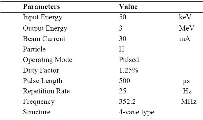
Table 1. The design specifications of the RFQ.
and Accelerating Section. The various studies which were performed for the design of the RFQ are described in the following sections.
2. Beam Dynamics Design
The beam dynamics design of an RFQ is performed keeping in view a given ion species, input energy, beam current and emittances, operating frequency, interelectrode voltage, through choosing proper dynamics parameters, to reach the requirement of output energy, beam current and emittances. The beam loss control and the minimization of the emittance growth are considered to be the main issues while optimizing the linac configuration and the operating parameters.
The input normalized root mean square (rms) emittance of beam from ion source is taken as 0.02 π cm-mrad. The initial particle distribution is selected to be 4-D Waterbag for which total emittance is equal to 6 times the total, normalized rms emittance.
Various RFQ design parameters are optimized and the effects of space charge, image charge and multipole terms of electric potential are also included in the calculation with the help of standard code PARMTEQM [3] for maximum transmission efficiency with minimum emittance growth. The variation of RFQ beam dynamics parameters along the length of RFQ is shown in Figure 1. The beam dynamics design for the ion beam, i.e. the design of the shape of the RFQ electrodes, results in a continuous change of aperture, vane modulation and cell length along the RFQ.
Intervane voltage is one of the very important parameters for the design and reliable working of RFQ. Higher intervane voltage results in higher energy gain, shorter cavity and better performance, but on the other hand it requires more RF power and face the danger of RF sparking. So the maximum vane voltage is decided by the Kilpatrick Criterion. In this design the peak electric field is limited to 1.7 times the Kilpatrick criterion. The intervane voltage is kept constant at 79.97 kV along the structure, so that adjusting the field distribution along the length will be easier [4,5].
Our RFQ design starts with an adiabatic radial matcher which transforms the dc input beam into a radially time-varying beam matched to the FODO focusing structure of the time-varying quadrupole field in the RFQ. In this design, the radial matching section (RMS) occupies six cells, each of length βλ/2 = 0.4391 cm, where β=v/c is the ratio of the particle velocity v to speed of light in vacuum c and λ is the free space rf wavelength; hence the total length of RMS is 2.6346 cm. In the RMS, the focusing strength ‘B’ is brought up from zero by ramping the vane tip radius ‘ ’ from large value down to average radius ‘
 ’ = 0.3495 cm without modulation
(m=1). The synchronous phase ‘ ’ is kept constant at -900, for which the separatrix has the largest phase width and the longitudinal acceptance is maximum.
In the RFQ, the next is the shaper section, following the RMS, which contains 75 cells. In the shaper section, the bunching process is initiated with a slow increase of stable phase from -900 to -830 and with a slow increase of
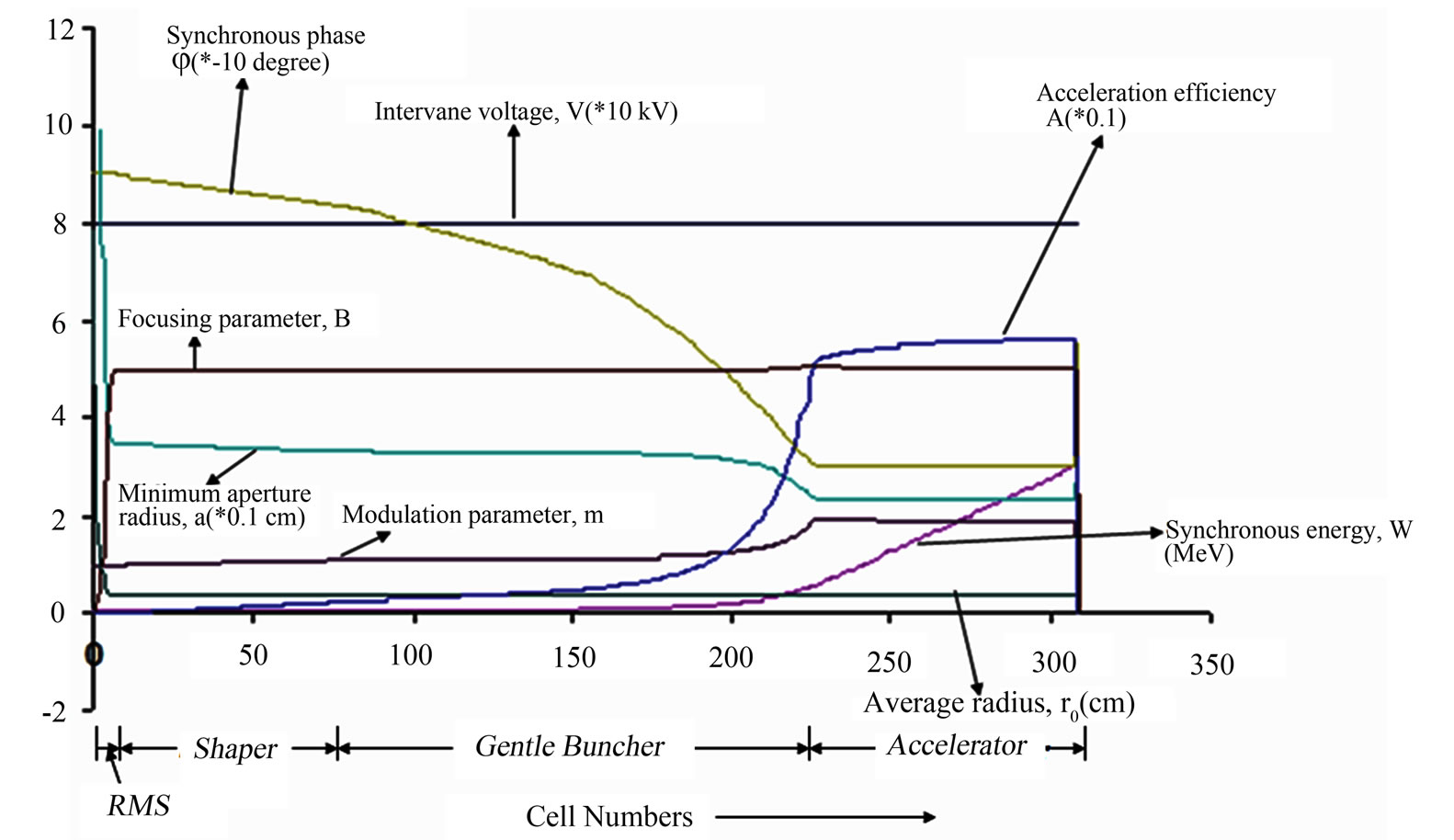
Figure 1. Variation of parameters along the length of RFQ.
modulation parameter ‘m’ from 1 to 1.1142 which increases the acceleration efficiency ‘A’ from zero (in the RMS) to 0.026. The energy of synchronous particle is slowly increased from 50 keV to 55 keV.
Downstream to shaper section, there is 145 cells long gentle buncher (GB) section which adiabatically bunch the beam. In the GB, longitudinal electric field, ‘Ez’ is turned on gradually by increasing the modulation index ‘m’ in a controlled fashion. The stable phase is gradually then increased to -300 and the modulation is increased to 1.9523. In the GB section, the parameters are chosen such as to keep bunching as well as to keep a nearly constant charge density for reducing the effect of spacecharge. The beam is brought to 560 keV and fully bunched at the end of GB section. The most critical point in the RFQ is the end of the buncher section where the beam energy is not significantly higher than at injection, but the bunch charge density is highest. This results in maximum space-charge force on the beam at the end of GB; therefore the aperture is reduced to its minimum value to have the maximum focusing strength.
After matching radially and longitudinally, the ion beam enters the accelerating section consisting of 81 cells. Here, synchronous phase ‘ ’, modulation ‘m’ and focusing parameter ‘B’ are kept nearly constant for high accelerating efficiency and to reach the final accelerating energy of 3 MeV.
After the accelerating section a transition cell of length 2.9083 cm is included. The purpose of the transition region is to end the RFQ vane tips with quadrupole symmetry, which eliminates the nonzero axial potential (and hence accelerating field) at the end of the RFQ vanes. Particles experience no energy change after the end of the vanes because there is no modulation (m = 1) in this region. The transition region also provides a convenient way to control the orientation of the output transverse phase-space ellipses, which eases matching the beam into a following accelerating structure or focusing channel.
Following the transition region, an exit fringe-field region is also included. The most important function of the exit fringe-field region is to provide a well-defined geometry at the end of the RFQ, where the RF fields are known and can be included in the beam-dynamics simulation by PARMTEQM. The fringe-field region consists of one cell having length 1.118 cm and also serves as a radial matching section at the end of the RFQ. This also insures the transport of the beam through the transverse RF focusing fields that exist in this region.
The average radius, ‘r0’, and the vane tip transverse radius of curvature, ‘ρ’ are kept constant for the ease of mechanical fabrication; and the ratio of the vane tip transverse radius of curvature to the average radius, ‘ρ/r0’, is kept constant to maintain a constant capacitance per unit length along the axis of RFQ [6,7].
The total 309 cells of all sections are combined to give the total length of 346.6316 cm for RFQ.
The main design parameters of this RFQ are listed in Table 2. In this table ‘εx,y,rms,n’ is representing the transverse normalized rms emittances and ‘εz,rms,n’ stands for the longitudinal normalized rms emittance. Figures 2 and 3 show the beam simulation results by PARMTEQM.
In the PARMTEQM, 10000 macroparticles are simulated and observed the dynamics along the length of RFQ. With the input transverse normalized rms emittance of 0.02π cm-mrad of beam, the output emittance is found to grow by less than 14% and the transmission efficiency of 98% with 10000 macroparticles is obtained.
Figure 2 shows the transverse (x vs xp and y vs yp, where x, y are the transverse beam size coordinates and
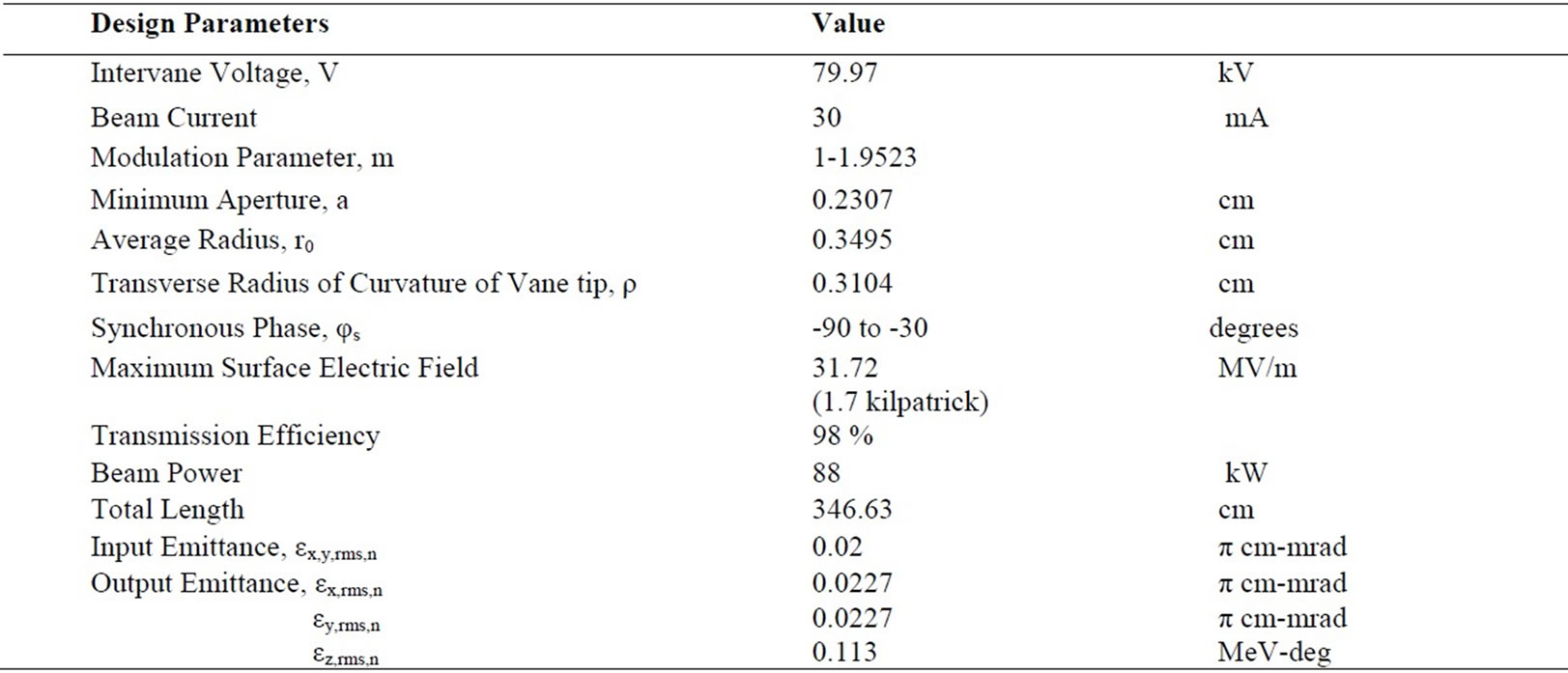
Table 2. The design parameters of the RFQ.
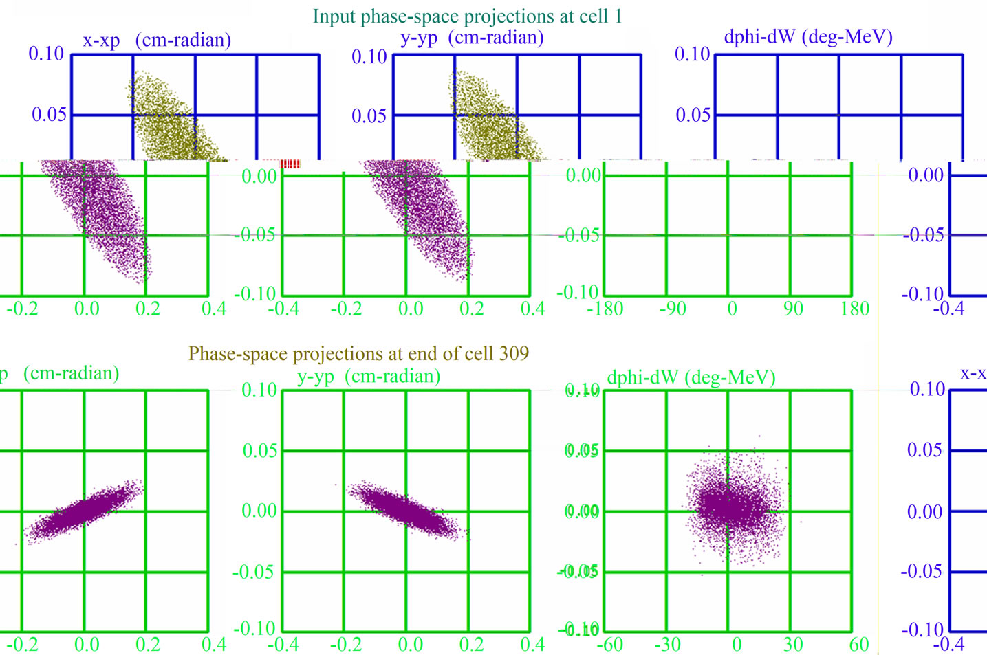
Figure 2. The phase-space projections at input of cell 1 and output of cell 309.
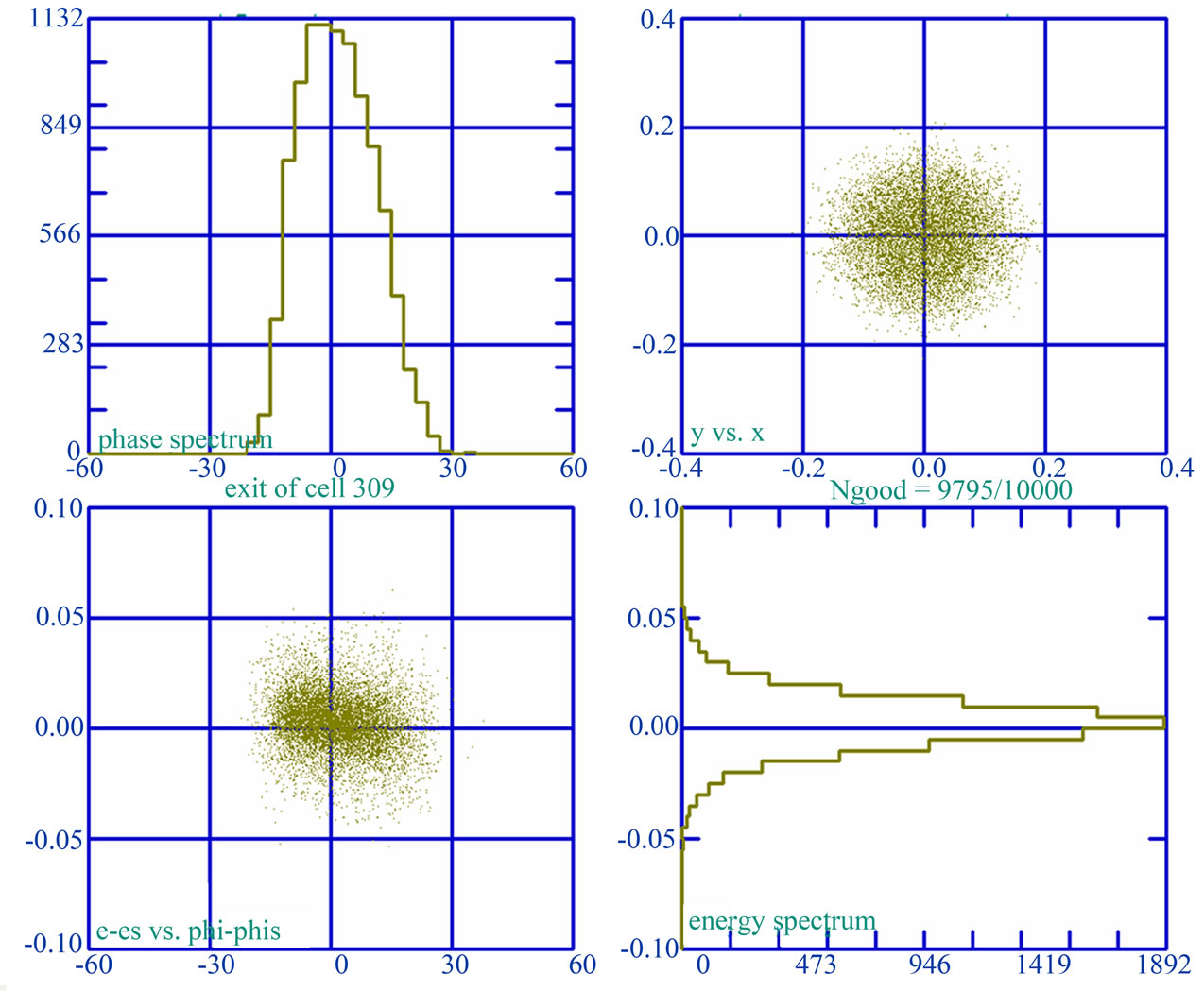
Figure 3. Phase spectrum (top left) and the energy spectrum (bottom right) at the exit of cell 309. The top right and the bottom left shows the distributions in x vs y and dw vs dphi respectively.
xp, yp are the transverse beam divergence coordinates) and longitudinal (dphi vs dw, where dphi and dw are the phase spread and energy spread of the particles respectively) phase space projections at the entrance and exit of RFQ. Here, the phase space projections are representing the unnormalized emittances. The unnormalized transverse emittance is reduced at the output of RFQ because of the reason that the divergences of the particles are reduced during longitudinal acceleration. The acceleration does not affect the normalized emittance. The initial longitudinal beam entering the RFQ has no phase space area because of zero energy spread. The bunching and acceleration of the beam takes place along the RFQ. As the bunch picks up energy spread, the separatrix height dw increases to contain the particle orbits, and the beam has a non-zero longitudinal emittance at the exit of RFQ.
Figure 3 shows the transverse (y vs x) and longitudinal (dw vs dphi) beam profiles; and the phase spectrum (number of macroparticles vs phase spread) and energy spectrum (number of macroparticles vs energy spread) at the output of RFQ. The transverse beam profile is showing the beam radius of ~1.6 mm which is calculated from the twiss parameters at the end of RFQ. It can be noticed from the spectrum that 98% transmitted particles are distributed around the peak at zero energy spread and zero phase spread.
3. Error Analysis of Input Beam Parameters
Transmission efficiency of RFQ depends on the various design parameters. In reality there are some fluctuations in the value of ion source parameters, beam parameters etc which greatly affect the transmission of the particles through RFQ. To set some tolerance limits on the various parameters, the error study [4] is performed. The study of the effect of errors on the beam dynamics of the 3 MeV RFQ is carried out with the help of code PARMTEQM. The variation of transmission efficiency is studied with the various effects, i.e. input beam displacement, beam angle divergence, voltage factor, input emittance, input energy deviation, input current etc. Figures 4-9 show the various effects. The acceptance criterion is taken as 95% transmission. Based on this criterion, the tolerance limits are set on the various parameters.
Figure 4 shows the variation of transmission effi-
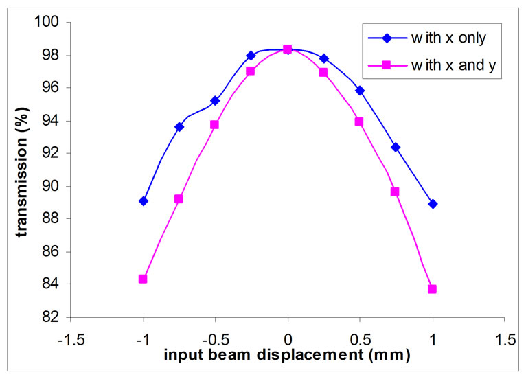
Figure 4. Transmission vs Input beam displacement.
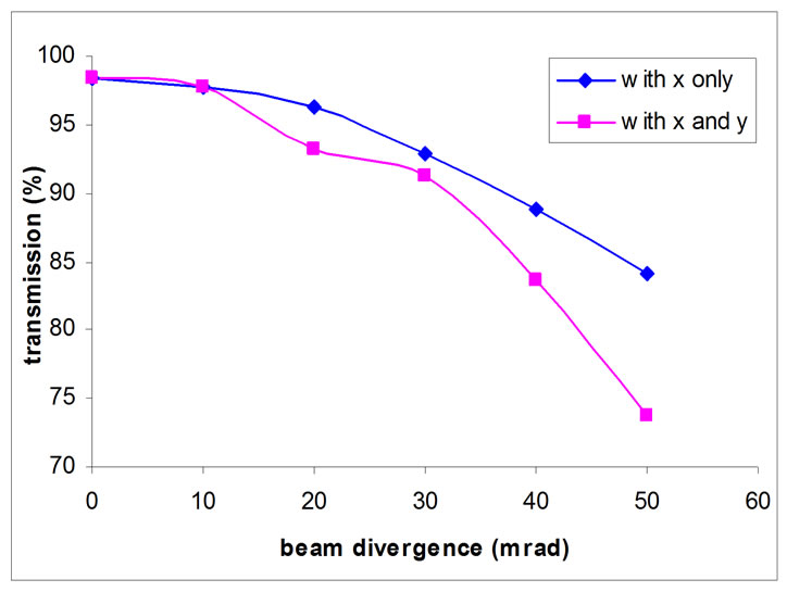
Figure 5. Transmission vs Beam divergence.
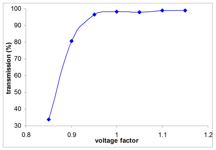
Figure 6. Transmission vs Voltage factor.
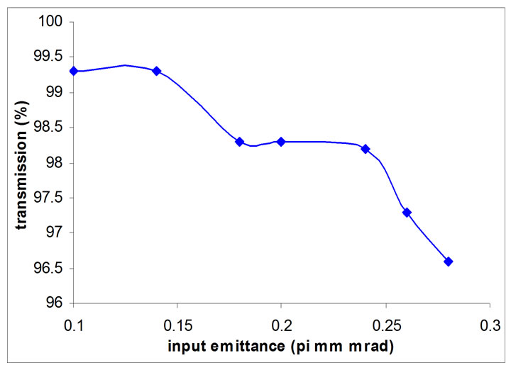
Figure 7. Transmission vs Input emittance.
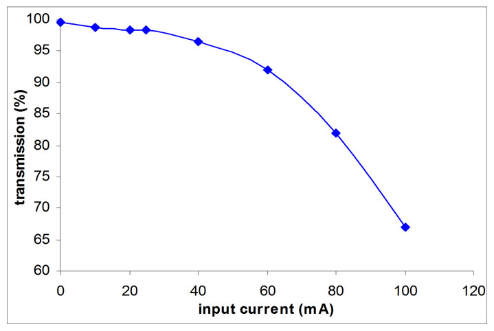
Figure 8. Transmission vs Input Current.
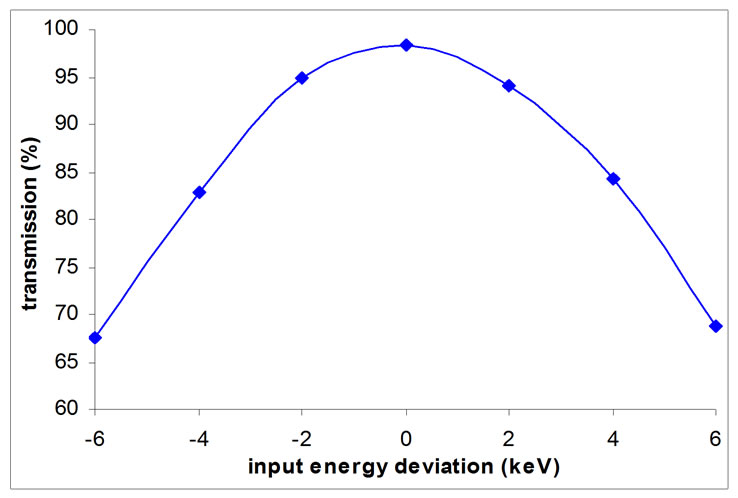
Figure 9. Transmission vs Input energy deviation.
ciency with the input beam displacement in transverse directions. With the displacement of beam the transmission efficiency goes down. From the graph shown, the input beam displacement of ± 500 μm is acceptable.
Figure 5 is the graph between transmission efficiency and beam angle divergence. As the angle of divergence increases, percentage transmission reduces. For obtaining the transmission more than 95%, beam angle divergence of ~15 mrad is acceptable.
Figure 6 shows the transmission efficiency vs the voltage factor. Voltage factor is a vane-voltage multiplier. It can be seen from the graph that below the value 0.95 of voltage factor the transmission reduces sharply, therefore the voltage factor has to be kept greater than 0.95 for better transmission.
From the graphs for transmission vs input emittance and current, which are shown in Figures 7 and 8 respectively, it can easily be observed that the transmission will be better for lower emittance and lower current. The input beam current upto ~50 mA is acceptable.
Figure 9 shows how transmission behaves with the variation in the energy of the beam coming to the input of RFQ. From the graph the input energy deviation of ± 2 keV is acceptable for the transmission greater than 95%.
4. Design of Two-Dimensional RFQ Cavity
For the designing of CW or pulsed structures, some parameters have to be optimized accordingly. The main consideration while designing the CW RFQ is to keep the power dissipation minimum. The lower power dissipation per unit length is required to ease the cooling. The power dissipation should be kept much below 1 kW/cm of the structure; otherwise cooling related problems will arise. Therefore, a lower vane voltage should be preferred for the high duty factor/CW operation, which results in low power dissipation per unit length. On the other hand, for the pulsed accelerators, there is no problem of cooling because power dissipation is reduced due to low duty factor. Since in our case, a pulsed beam is needed from linac, we need not worry about the power dissipation and cooling problems. However, we have paid much attention on the alignment and tolerance limits, for fabrication purpose, which become too stringent at higher frequencies, as in this case 352.2 MHz. The RFQ cavity is designed with the 2-D simulation code SUPERFISH [8].
The two-dimensional cavity is designed in SUPERFISH and the various geometrical parameters are optimized to obtain the designed frequency of 352.2 MHz. Figure 10 is showing the cross-section of one quadrant of RFQ cavity and Figure 11 is highlighting the details near the vane-tips. The geometrical parameters, i.e., average bore radius ‘r0’, vane-tip transverse radius of curvature ‘ρ’ are determined from the beam dynamics design and used in SUPERFISH for cavity design. The voltage difference between adjacent vane tips (at the peak of the rf waveform) is called the gap voltage ‘Vg’. The gap voltage is set to 79.97 kV to normalize the fields.
In Figure 11, the lower left corner is the RFQ beam axis. The unmachined tip of the vane is often referred as the “vane blank.” Before the numerically controlled machining of the tip, the vane blank would have a rectangular cross section in these views. The break-out angle ‘abk’ for the tool bit cutting the vane is selected to be 15 degrees. Thus, the half width ‘BW’ of the vane blank must always exceed the vane-tip radius of curvature ‘r’ for cross sections at any longitudinal position along the vane, otherwise it would be very difficult to machine the tip without leaving a ridge along one side of the vane. A raised ridge would be especially undesirable because of the high electric field near the tip. Therefore, the vane blank half width is optimized to be 0.6 cm. The vane blank depth ‘BD’ is the distance from the RFQ axis to the vertex of angle ‘a1’. At this point, the vane width increases at distances farther from the RFQ axis until it reaches the limit set by ‘Ws’, the half width of the vane shoulder. The shoulder segment of length ‘Ls’ is parallel to the vane axis. At the end of the shoulder segment farthest from the RFQ axis is the vertex of angle ‘a2’. Again, the vane width increases farther from the RFQ axis until it reaches the limit set by ‘Wb’, the half width of the vane base.
The various geometrical parameters are listed in Table 3.
With these geometrical parameters, a quadrant of RFQ cavity was designed. After setting these parameters, the appropriate boundary conditions were applied to calculate the quadrupole (TE210-like) and the dipole (TE110- like) modes. For the quadrupole mode, the Neumann boundary condition was applied to upper and right edges and the Dirichlet boundary condition was applied to lower and left edges in the problem geometry. The quadru-
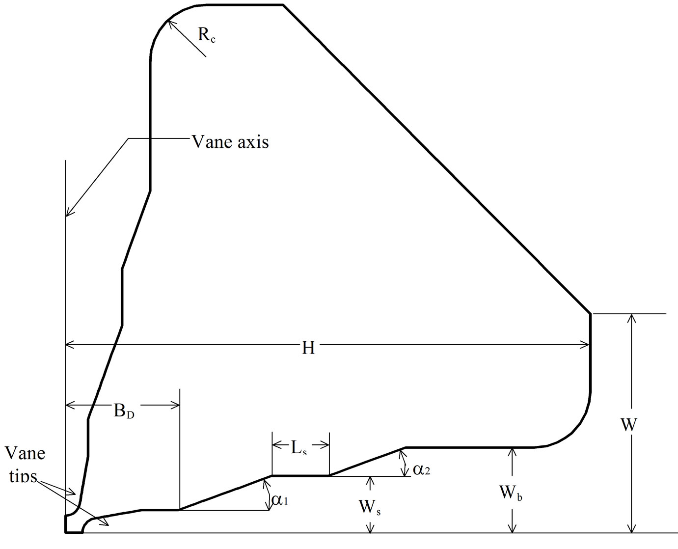
Figure 10. Cross-section of one quadrant of an RFQ cavity.
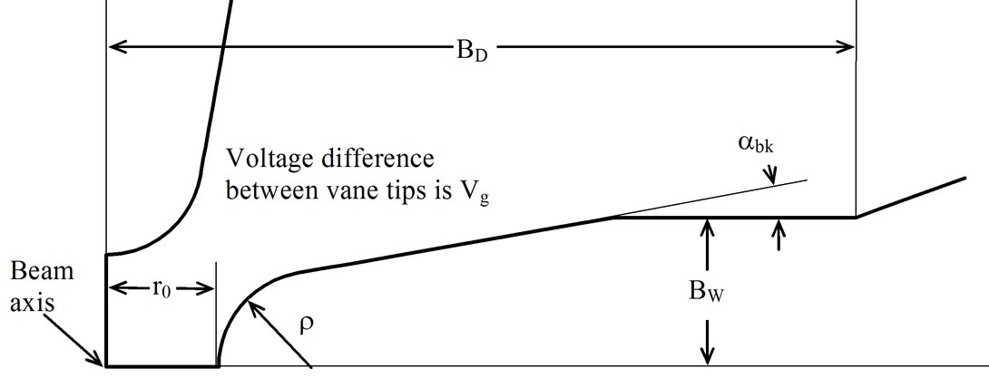
Figure 11. Details near the vane tips for the RFQ quadrant.
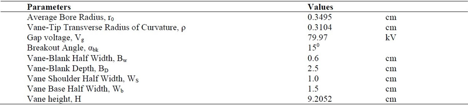
Table 3. Geometrical parameters of the RFQ.
pole mode frequency of the cavity was optimized at 352.1996 MHz; and the quality factor for this mode was calculated to be 10030. To calculate the dipole mode frequency, the left edge of the problem geometry was changed to Neumann boundary. The adjacent dipole mode frequency was obtained as 342.0099 MHz.
The total power dissipation on the walls per quadrant is 230 W/cm, hence the total structure power loss for whole the RFQ cavity of the length 346.6316 cm was calculated to be 319 kW. Since the beam power from the beam dynamics calculation was found to be 88 kW; thus the total power dissipation in the RFQ is the sum of structure power dissipation and beam power, hence calculated to be 407 kW. This power dissipation is calculated for the CW beam. In our case of pulsed RFQ, the power dissipation will be greatly reduced by the duty factor.
The frequency sensitivities in horizontal and vertical directions are much higher at the vane-tips than any other points, so the special care has to be taken for the mechanical design near vane-tips.
The two-dimensional design parameters of the RFQ are listed in Table 4.
5. Three-Dimensional RFQ Cavity Design
To look into the more details of electromagnetic field properties required by the beam dynamics in the RFQ, the three-dimensional model of RFQ cavity was prepared in CST Microwave Studio code [9].
After the beam dynamics design, done in PARMTEQM code, the electromagnetic design of RFQ cavity was done in two-dimensional code SUPERFISH. But for the detailed study of electromagnetic design of RFQ, a three-dimensional model was required. Due to the complexity of the RFQ structure, a three-dimensional model with large mesh ratio was required to adequately model the necessary details of the structure. To solve the model with large mesh ratio, an accurate enough threedimensional code is needed to predict the correct resonant frequency and electromagnetic field of the structure. CST Microwave Studio code is a three-dimensional electromagnetic code which is accurate enough due to Perfect Boundary Approximation (PBA) technique. The threedimensional model of RFQ was prepared in CST MWS as per the dimensions optimized from two-dimensional code SUPERFISH. The unmodulated RFQ cavity model is shown in Figure 12.
To determine the resonant frequency of the structure, the right boundary conditions should be applied. In the transverse directions (x and y), the boundaries are elec-
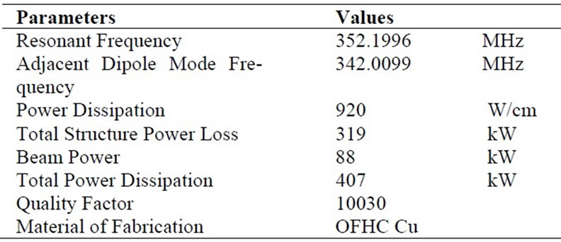
Table 4. Two-dimensional design parameters of RFQ.
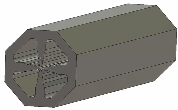
Figure 12. The unmodulated RFQ model.
tric (Et = 0); and in the longitudinal direction (z), the magnetic boundaries (Ht = 0) are applied. RFQ is a symmetric structure; it has two symmetry planes at the axis. To save the memory and the CPU time, only a quadrant of the structure was simulated. To simulate the quadrupole mode, the magnetic boundary conditions (Ht = 0) were put at the both xzand yzplanes. For calculating the dipole mode, the boundary conditions at xzand yzplanes should not be same, which means that either put electric boundary in xz-plane and magnetic boundary in yz-plane, or magnetic boundary in xz-plane and electric boundary in yz-plane [10].
The quadrupole mode and dipole mode frequencies were calculated with the eigenmode solver. The calculated frequencies from CST MWS code were close to those calculated from two-dimensional SUPERFISH code but not exactly matching because of limitation of 3D code in handling a large number of mesh points. Due to this reason the operating quadrupole mode frequency for the 3-dimensional unmodulated RFQ structure was considered to be 350.913 MHz optimized from CST MWS.
5.1. Study of Vane-Ends
The RFQ resonator has, of course, to be closed at both ends. In this situation, the longitudinal magnetic field will be perpendicular to the end cover; but to satisfy the boundary condition, the magnetic field must be parallel to the end cover. For the solution of this problem the vane-ends should be designed in such a way so that the magnetic field must turn round and this change of direction must not influence the constant vane potential. Therefore, the vanes should not extend right up to the end covers and, in addition the cut-backs are given at the both ends, entrance and exit, to facilitate the Uturn of the magnetic field. The ‘end region’ can also be represented by an equivalent circuit shown in Figure 13. It must resonate at the quadrupole frequency, i.e. , which is a condition necessary to keep the vane potential constant. Here L and C are representing the inductance and capacitance respectively of the RFQ
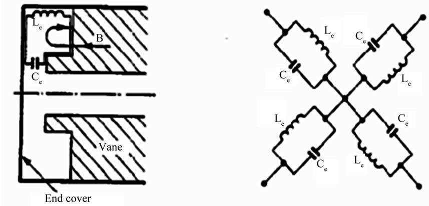
Figure 13. Equivalent circuit of RFQ vane-ends.
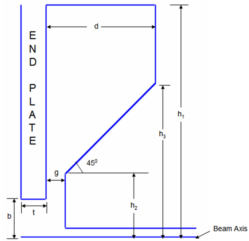
Figure 14. Cutback dimensions at the entrance and exit of RFQ.
cavity, whereas Le and Ce stand for vane-end region.
Figure 14 is showing the parameters optimized for cut-back at the entrance and exit ends of RFQ [11,12]. Keeping the value of g, h1 and slope of 450 constant, we optimized the entrance and exit cutbacks by varying the parameters, i.e., cutback thickness d, end plate thickness t, beam port radius b and heights h2, h3. The optimized values of the parameters are shown in the Table 5.
These parameters are optimized such that these end cells resonate at the quadrupole frequency of 350.913 MHz.
6. Conclusions
An RFQ is designed for 352.2 MHz operating frequency and 30 mA beam current of H- particles, which has to be accelerated from 50 keV to 3 MeV, to serve as a low energy front-end injector of 100 MeV linac.
The beam dynamics study of RFQ is done with the help of PARMTEQM simulation code. The various beam
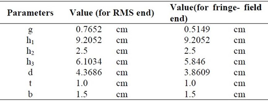
Table 5. The geometric parameters of the end cells.
dynamics parameters are optimized for the maximum transmission of particles and the minimum emittance growth while beam passes through RFQ. With the optimization of various parameters, the transmission efficiency of 98% is achieved with less than 14% emittance growth at the exit of RFQ.
Due to fluctuations in various parameters, the transmission of the particles is greatly affected, so the error analysis is performed to study the effect of these parameters on the transmission efficiency.
For the electromagnetic study of RFQ, the two-dimensional cavity is designed with the help of SUPERFISH simulation code. The various geometrical parameters of RFQ cavity are optimized to attain the desired operating frequency 352.2 MHz. The total power dissipation of ~407 kW and the quality factor of 10030 are calculated of the RFQ cavity for the quadrupole mode. The nearest dipole mode frequency is obtained at 342.0099 MHz. For the detailed electromagnetic analysis of fields inside the cavity, a three-dimensional model of RFQ cavity was created and analysed in CST Microwave Studio as per the geometric dimensions optimized from the PARMTEQM and SUPERFISH code. In the end, to make the U-turn of magnetic field and to flatten the field in the four quadrants the cut-backs at the both ends, entrance and exit, are studied. Based on these studies, the fabrication of a prototype RFQ has been started.
7. Acknowledgements
We thank Dr. P. D. Gupta (Director, RRCAT) and Dr. P. Singh (Incharge, IAP, RRCAT) for the constant encouragement and keen interest in the project. We are also thankful to Mrs. Nita Kulkarni, P. K. Jana and Chirag Patidar for the useful discussions.
REFERENCES
- T. P. Wangler; “Principles of RF Linear Accelerators,” John Wiley & Sons, New York, 1998.
- J. W. Staples, “RFQsAn Introduction,” LBL-29472.
- K. R. Crandall, T. P. Wangler, L. M. Young, J. H. Billen, G. H. Neuschaefer and D. L. Schrage, “RFQ Design Codes,” LA-UR-96-1836.
- Z. H. Luo, X. L. Guan, S. N. Fu, L. L. Wang and Z. Y. Guo, “Beam Dynamics Design and Error Study of the 5MeV RFQ,” Proceedings of the Second Asian Particle Accelerator Conference, Beijing, 17-21 September 2001, pp. 439-441.
- H. J. Kwon, Y. S. Cho, J. H. Jang, H. S. Kim and Y. H. Kim, “Fabrication of the PEFP 3 MeV RFQ Upgrade,” Proceedings of 2005 Particle Accelerator Conference, Knoxville, Tennessee, 16-20 May 2005, pp. 3010-3012.
- J. M. Han, Y. S. Cho, B. J. Yoon, B.H. Choi, Y. S. Bae, I. S. Ko, and B. S. Han, “Design of the KOMAC H+/H- RFQ Linac,” Proceedings of XIX International Linear Accelerator Conference, Illinois, 23-28 August 1998, pp. 774-776.
- H. F. Ouyang, S. Fu, “Study of CSNS RFQ Design,” Proceedings of LINAC 2006, Knoxville, Tennessee, 21- 25 August 2006, pp. 746-748.
- J. H. Billen and L. M. Young, “Poisson Superfish,” LA-UR-96-1834.
- CST Studio Suite, “CST Microwave Studio,” 2008. http:// www.cst.com
- D. Li, J. W. Staples and S. P. Virostek, “Detailed Modeling of the SNS RFQ Structure with CST Microwave Studio,” Proceedings of LINAC 2006, Knoxville, Tennessee, 21-25 August, 2006, pp. 580-582.
- H. F. OuYang, T. G. Xu, X. L. Guan, Z. H. Luo and W. W. Xu, “The Study on RF Field of an RFQ,” Proceedings of the Second Asian Particle Accelerator Conference, Beijing, 17-21 September 2001, pp. 722-724.
- G. Romanov and A. Lunin; “Complete RF Design of the HINS RFQ with CST MWS and HFSS,” Proceedings of LINAC08, Victoria, BC, 29 September-3 October 2008, pp. 163-165.