Int'l J. of Communications, Network and System Sciences
Vol.6 No.11(2013), Article ID:39718,6 pages DOI:10.4236/ijcns.2013.611049
PSO for CWSN Using Adaptive Channel Estimation*
Electrical Engineering Department, The University of Jordan, Amman, Jordan
Email: rahhal@ju.edu.jo
Copyright © 2013 Jamal S. Rahhal. This is an open access article distributed under the Creative Commons Attribution License, which permits unrestricted use, distribution, and reproduction in any medium, provided the original work is properly cited.
Received October 31, 2013; revised November 15, 2013; accepted November 17, 2013
Keywords: CWSN; MIMO; CSI; LMS; Adaptive Channel Estimation; Particle Swarm
ABSTRACT
Wireless Sensor Network (WSN) is used in various applications. A main performance factor for WSN is the battery life that depends on energy consumption on the sensor. To reduce the energy consumption, an energy efficient transmission technique is required. Cluster Wireless Sensor Network (CWSN) groups the sensors that have the best channel condition and form a MIMO system. This leads to enhancing the transmission and hence reducing energy consumed by the sensor. In CWSN systems multiple signals are combined at the transmitter and transmitted by using multiple antennas according to channel condition. CWSN requires a good estimation of the Channel State Information (CSI) to implement a powerful and efficient system. Channel Estimation technique should be used to better form the CWSN and make use of the MIMO features. Adaptive Channel Estimation (ACE) is used to enhance the BER performance of the CWSN by utilizing the retransmission feature devised in this paper and feeding the CSI obtained to further enhance the clustering algorithm. We use Particle Swarm Optimization (PSO) algorithm to find the optimal cluster members according to a fitness function that derived from the channel condition. Too many calculations and operations are required in exhaustive search algorithms to form the optimal cluster arrangement. It shows that optimal cluster formation can be implemented fast and efficiently by using the PSO.
1. Introduction
Cluster Wireless Sensor Network (CWSN) is defined as spatially distributed autonomous groups of sensors to monitor physical or environmental conditions. The development of wireless sensor networks is motivated by many industrial and civilian application areas, such as environment, pollutants, medicine, vehicles, energy management, inventory control, home and building automation, homeland security and others [1-10]. Performance of WSN is measured and optimized based on various criteria, such as capacity, bit error rate, SNR, Cross-layer Optimal Scheduling, power requirements, security and robustness. The performance of CWSN depends on the quality of decision parameters in forming the cluster and detecting the data. These parameters include the CSI such that the cluster can be formed by selecting the best channel condition among the sensors for clusters forming a virtual MIMO channel. They select the cluster head if only one sensor from each cluster is transmitting the data as in the dense wireless sensor network.
Channel Estimation is the process of characterizing the effect of the physical medium on the input signals. It is an important process for wireless systems so that a receiver can detect the data sent over by the transmitter. In training sequence based on estimation, Channel State Information (CSI) is estimated based on the training sequence which is known to both transmitter and receiver. Blind channel estimation methods avoid the use of pilot symbols, which makes them good candidates for achieving high spectral-efficiency such as equalizers [11,12].
Channel estimation insures better power distribution among the transmitting sensors. In CWSN only good channels are maintained and they form the clusters. The estimation of CSI is therefore critical to operate the network at the lowest possible power consumption. CSI is usually random in nature and hence many techniques are used to estimate them. In efficient transmission we need to know a good estimate of CSI such that the transmitter and receiver can compensate for the loss in signal energy and choose the optimal weights for the transmitted signals. This leads to better overall systems performance including saving battery life [13-18].
Adaptive Channel Estimation (ACE) shows better performance in receiving data, since the adaptation mechanism follows the channel variation and hence, closer CSI is to exact ones that can be estimated. One of low-complexity and stable adaptive channel estimation approaches is the least mean square (LMS)-based ACE. In this paper we use the retransmission feature of the CWSN to get a pre-estimate of the received data and then use the LMS algorithm to estimate the CSI each time when a transmission occurs.
2. System Description
Cluster Wireless Sensor Network (CWSN) is formed as a cluster of sensors that satisfying a channel condition criteria to form a virtual MIMO system. In Wireless Networks the use of reliable and energy efficient transmission is critical to most applications. The battery life is mostly dependent on the transmitted RF power. Therefore, using a transmission scheme that has acceptable BER at the lowest possible SNR is the goal of current research in the WSN field. The MIMO system can provide such feature since it makes use of transmission diversity and hence improves BER performance. The WSN is suitable to form a MIMO system since it has many transmitters and many receivers. The utilization of MIMO system requires a good knowledge of Channel State Information (CSI) that is required in forming the best possible MIMO system among the sensors as shown in Figure 1.
In this paper we devise an estimation based on adaptive iterative technique that utilizes the CWSN capabilities to best estimate the channel matrix. The iteration makes use of the cluster nature; such that, in each cluster the sensors transmit their data to the master unit and at the same time collect the signals from each others. Then the collected signals are retransmitted again to the master unit. The adaptive estimator calculates the CSI for the cluster and reevaluates the cluster condition; such that new members can be added or deleted from the cluster (reforming the clusters).
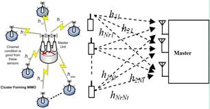
Figure 1. A cluster forming virtual mimo channel.
To form the cluster we need the knowledge of CSI; such that, only sensors with good channel condition are grouped in one cluster. This requires a big processing power since the total number of sensors usually huge. To reduce the calculations in forming the cluster we might search in only sup set of the overall CSI values depending on the sensors locations. Here we propose the use of PSO algorithm to form the cluster.
PSO is a population based stochastic optimization technique inspired by social behavior of bird flocking or fish schooling. The system is initialized with a population of random solutions and searches for optima by updating generations. In PSO, the potential solutions, called particles, fly through the problem space by following the current optimum particles. Each particle keeps track of its coordinates in the problem space which are associated with the best solution (fitness) it has achieved so far. This value is called pbest. Another "best" value that is tracked by the particle swarm optimizer is the best value, obtained so far by any particle in the neighbors of the particle. This location is called lbest. When a particle takes all the population as its topological neighbors, the best value is a global best and is called gbest.
The particle swarm optimization concept consists of, at each time step, changing the velocity of accelerating each particle toward its pbest and lbest locations. Acceleration is weighted by a random term, with separate random numbers being generated for acceleration toward pbest and lbest locations. PSO has been successfully applied in many research and application areas. It is demonstrated that PSO gets better results in a faster, cheaper way compared with other methods. In order to illustrate the steps of the PSO algorithm for our problem, two parts can be classified [19,20]:
2.1. Parameter Settings
For parameter initialization of the PSO:
• Set the system parameters.
• Set appropriate level step inputs to the system.
• Simulate the outputs with a suitable sampling time.
• Set the PSO parameters:
° The size of the particle, P.
° The number of particles in the swarm, M.
° The counter of iteration ( , Lmax).
• Definition of the solution space: A reasonable range for the parameters should be chosen. This requires specifications of the minimum and maximum values for each parameter.
• Definition of a fitness function: This step is the link between the optimization algorithm and the physical problem in hand.
2.2. Main Steps of the PSO Algorithm
The main steps of the proposed PSO algorithm are summarized as following:
1) Initialization
The PSO starts by randomly initializing the position matrix X, the velocity matrix V and the personal best matrix P, of each particle in the swarm such that:
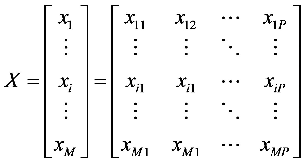 (1)
(1)
and the velocity matrix is:
 (2)
(2)
The personal best position can be defined by the matrix:
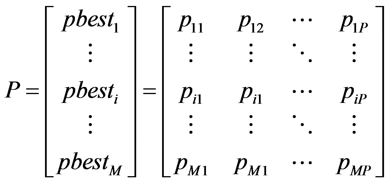 (3)
(3)
The global best solution gbest is the row of personal best matrix P with the best fitness function given as:
 (4)
(4)
In most cases, the initial position is the only location encountered by each particle at the start of the algorithm. Hence, it will be regarded as the particle’s respective personal best.
2) Particle Updating
The particles of each iteration are moved into the solution space. The algorithm will act on each particle such that each particle will move in a direction to improve its fitness function. The following steps summarize the action encountered for each particle in the swarm:
a) Particle’s Velocity Updating
The particle’s velocity will be updated according to three vector elements: the first is the relative location to its corresponding pbesti; the second is its relative location to gbest; and the third vector is a scaled factor of the old velocity. For each particle, the velocity update is obtained based on the following equation:
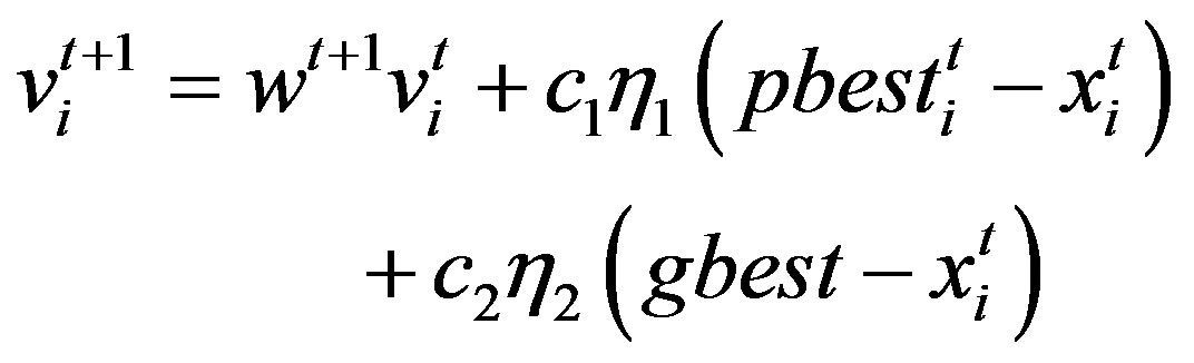 (5)
(5)
The superscript t + 1 and t refer to the time index of the next and the current iterations.  and
and  are two uniformly random numbers in the interval [0,1]. A good choice for c1 and c2 are both 2.0. The parameter wt is a number called the inertial weight which is a scaling factor of the previous velocity of the particles. It has been demonstrated that PSO algorithms converges faster if w is chosen to be linearly damped with iterations [18,19]. A good choice to start with is w1 = 0.9 at the first iteration and linearly decreases to wLmax = 0.4 with the last iteration.
b) Particles Movement Updating
Once the velocity of each particle is determined, the position will be updated:
 (6)
(6)
For simplicity,  is chosen to be unity.
c) Fitness Evaluation pbest
The fitness function of the new position is compared with the fitness function of pbest. This is performed based on the condition that if fitness( ) < fitness(pbesti) then pbesti =
 .
.
d) Fitness Evaluation gbest
The fitness function of the new position is compared with the fitness function of gbest. This is performed based on the condition that if fitnes ( ) < fitness(gbest) then gbest =
 .
.
e) Iteration
Repeat (a), (b), (c) and (d) for the whole M particles.
3) Termination
Check if maximum iteration reached or a specified termination criterion is satisfied. Then, the solution is gbest. Otherwise, update w and go to the next iteration. Implementing this algorithm to find the optimal cluster arrangement needs to define the fitness function. The fitness function is derived from the estimated CSI as follows: The sensor transmits its signals through the channel to the master unit and the received signals at the master unit are combined through multiple antennas. In matrix form we can write the transmitted signals for all sensors in a cluster as:
 (7)
(7)
where:
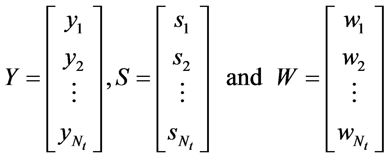 (8)
(8)
where yn is the nth sensor signal, sn is the physical quantity and wn is an iid  acquisition noise.
The transmitted signals are passed through a fading channel that we assume as flat Rayleigh fading channel since the transmission is usually narrow band. The received signals at the main unit can be written in matrix form as:
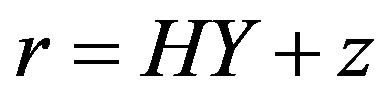 (9)
(9)
where:
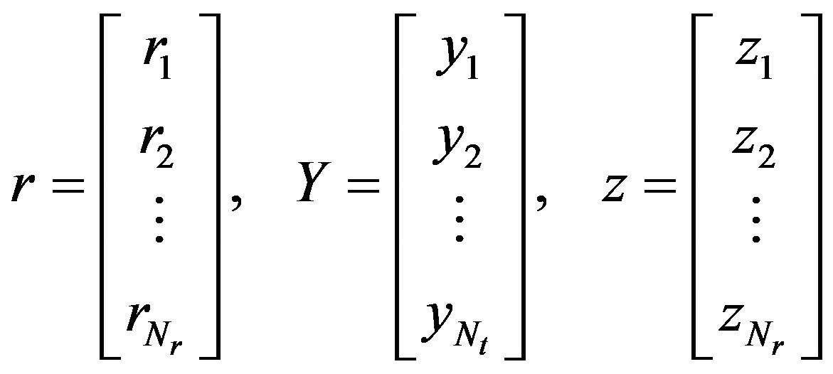 (10)
(10)
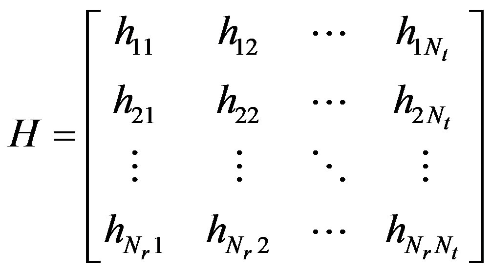 (11)
(11)
hmn is the nth sensor to the mth receiving antenna channel path gain, yn is the transmitted signal and z is a noise signal with zero mean and covariance matrix of Vzz. To detect the signal yn we use constraint estimation as:
 (12)
(12)
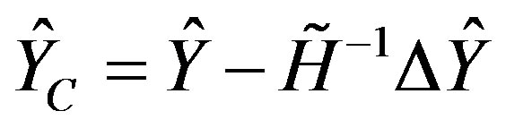
where the constraint is given by:
 (13)
(13)
where  are the first and the second estimate of the received signal, the estimated inverse channel matrix is given by:
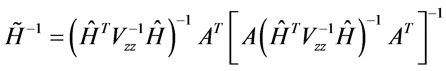 (14)
(14)
here  is the least mean square (LMS) estimate of the channel matrix.
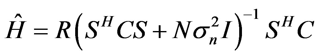 (15)
(15)
where S and R are the first and the second received symbol matrix respectively, C is the covariance channel matrix and  is the noise variance. To get the second estimate, each sensor in the cluster retransmits all the received signals from other sensors to the master unit.
The fitness function can be derived as the Condition Number (CN) of the estimated channel matrix. The CN measures the goodness and stability of the channel matrix, as it becomes closer to unity, the channel matrix becomes more stable and the reception becomes less sensitive to estimation errors. CN of the channel matrix defined as:
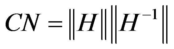 (16)
(16)
And the fitness function is given as:
 (17)
(17)
In the following we use MatLab to calculate the optimal cluster formation and performance for some examples using the PSO algorithm.
3. Simulation Results
A CWSN is simulated using the PSO clustering procedure described in the previous section. A simulation of 500 randomly deployed sensors and 50 master units each equipped with 10 receiving antennas forming the CWSN system as shown in Figure 2. The simulation is done by randomly deployed the 550 sensors then assuming the channel matrix for the whole 550 sensors that represent a Rayleigh fading channel.
Applying PSO algorithm by selecting the 50 master units among the 550 sensors. The position matrix X initialized to contain large numbers representing large CN, the velocity matrix V initialized to 1 and the personal best position matrix P initialized to large numbers. Initialize the parameters: p = 10, M = 500 and Lmax = 10. The first optimization round finds the optimal first cluster and other rounds finds the optimal clusters for the other master units.
Simulating the optimized system by:
1) Transmitting data.
2) Changing the channel randomly every 100 transmission intervals.
3) Estimation the channel matrix for each cluster.
4) Reform the clusters using PSO algorithm.
5) If maximum data size is not reached, go to (1).
Figure 3 shows the average BER as simulated by transmitting 100,000 data bits from each sensor.
Energy efficiency comes from the combination of good channel selection and MIMO system, such that lowering the BER allows the network to operate at lower transmitted power and hence, less energy is required at the sensor node. This condition can be maintained through the cluster
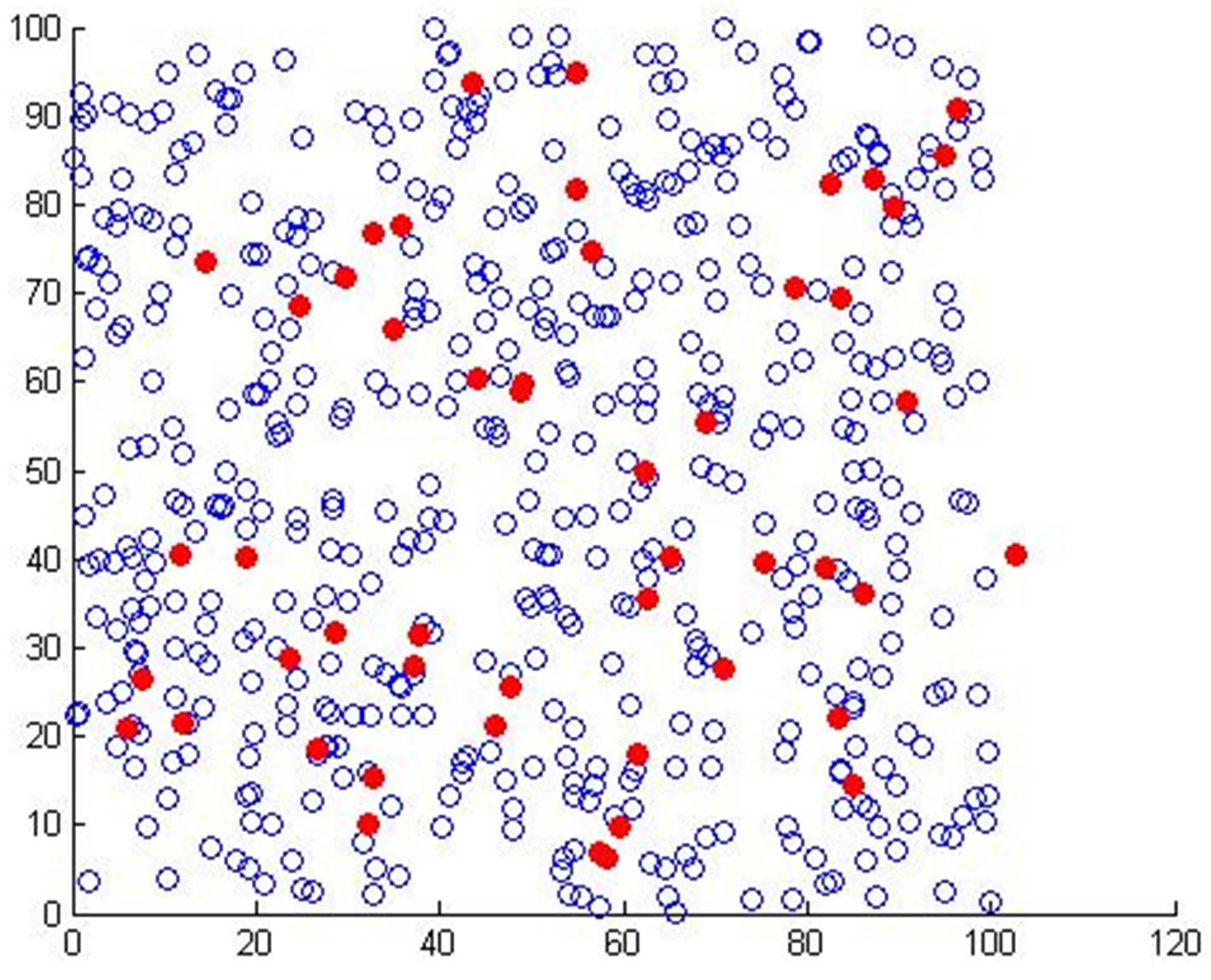
Figure 2. A 500 randomly deployed sensors (empty circles) and 50 master units (filled circles).

Figure 3. BER vs SNR for the simulated system with and without estimation.
selection devised in this paper and the adaptation process to maintain optimal configuration.
4. Conclusion
The proposed system has showed an opportunity to enhance the wireless sensor network by constructing a virtual MIMO system from signal repetition emitted from each sensor combined with good channel selection. Adaptive channel estimation provides a better signal detection and at the same time makes sure that the transmitted power from each sensor is reduced. The proposed method requires more signal processing at the master units to keep the sensor units at low complexity since the sensor nodes only need to retransmit the data and then arrive at its terminal. Finally, we can see that the clustering technique based on PSO algorithm used in this paper will maintain only the good conditioned channels; therefore, better BER and stability are obtained. This is shown by simulation.
REFERENCES
- J. Rahhal, “Wireless MIMO Sensor Network with Power Constraint WLS/BLUE Estimators,” Wireless Personal Communications, Vol. 63, No. 2, 2012, pp. 447-457. http://dx.doi.org/10.1007/s11277-010-0142-1
- I. Mansour, J. S. Rahhal and H. Farahneh, “Two Slot MIMO Configuration for Cooperative Sensor Network,” International Journal of Communications, Network and System Sciences, Vol. 3, No. 9, 2010, pp. 750-754.
- S. Cui and A. Goldsmith, “Energy-Efficiency of MIMO and Cooperative MIMO Techniques in Sensor Networks,” IEEE Journal on Selected Areas in Communications, Vol. 22, No. 6, 2004, pp. 1089-1098. http://dx.doi.org/10.1109/JSAC.2004.830916
- E. Uysal-Biyikoglu and A. El Ga, “On Adaptive Transmission for Energy Efficiency in Wireless Data Networks,” IEEE Transactions on Information Theory, Vol. 50, No. 12, 2004, pp. 3081-3094. http://dx.doi.org/10.1109/TIT.2004.838355
- G. Thatte and U. Mitra, “Sensor Selection and Power Allocation for Distributed Estimation in Sensor Networks: Beyond the Star Topology,” IEEE Transactions on Signal Processing, Vol. 56, No. 7, 2008, pp. 2649-2661.
- S. Valentin, et al, “CooperativeWireless Networking Beyond Store-and-Forward: Perspectives in PHY and MAC Design,” Wireless Personal Communications, Vol. 48, No. 1, 2009, pp. 49-68.
- R. Krishna, Z. Xiong and S. Lambotharan, “A Cooperative MMSE Relay Strategy for Wireless Sensor Networks,” IEEE Signal Processing Letters, Vol. 15, 2008, pp. 549-552. http://dx.doi.org/10.1109/LSP.2008.925751
- P. Clarke and R. C. de Lamare, “Joint Transmit Diversity Optimization and Relay Selection for Multi-Relay Cooperative MIMO Systems Using Discrete Stochastic Algorithms,” IEEE Communications Letters, Vol. 15, No. 10, 2011, pp. 1035-1037. http://dx.doi.org/10.1109/LCOMM.2011.082611.102262
- P. Clarke and R. C. de Lamare, “Transmit Diversity and Relay Selection Algorithms for Multirelay Cooperative MIMO Systems,” IEEE Transactions on Vehicular Technology, Vol. 61, No. 3, 2011, pp. 1084-1098. http://dx.doi.org/10.1109/TVT.2012.2186619
- M. K Gowda and K. K. Shukla, “Energy and Throughput Optimized, Cluster Based Hierarchical Routing Algorithm for Heterogeneous Wireless Sensor Networks,” International Journal of Communications, Network and System Sciences, Vol. 4, No. 5, 2011, pp. 335-344.
- J. Proakis, “Digital Communications,” 4th Edition, McGraw-Hill, New York, 2001.
- M. K. Simon and M.-S. Alouini, “Digital Communication over Fading Channels,” 2nd Edition, John Wiley, New York, 2005.
- F. Sanzi, J. Sven and J. Speidel, “A Comparative Study of Iterative Channel Estimators for Mobile OFDM Systems,” IEEE Transactions on Wireless Communications, Vol. 2, No. 5, 2003, pp. 849-859. http://dx.doi.org/10.1109/TWC.2003.817436
- L. Q. Zhao, L. Guo, C. Li and H. L. Zhang, “An Energy-Efficient MAC Protocol for WSNs: Game-Theoretic Constraint Optimization with Multiple Objectives,” International Journal of Communications, Network and System Sciences, Vol. 1, No. 4, 2009, pp. 358-364.
- T. Wang, R. C. de Lamare and P. D. Mitchell, “Low- Complexity Channel Estimation for Cooperative Wireless Sensor Networks Based on Data Selection,” IEEE Vehicular Technology Conference (VTC), Taipei, 16-19 May 2010, pp. 1-5.
- P. Li, R. C. de Lamare and R. Fa, “Multiple Feedback Successive Interference Cancellation Detection for Multiuser MIMO Systems,” IEEE Transactions on Wireless Communications, Vol. 10, No. 8, 2011, pp. 2434-2439. http://dx.doi.org/10.1109/TWC.2011.060811.101962
- R. C. de Lamare and R. Sampaio-Neto, “Adaptive ReducedRank Equalization Algorithms Based on Alternating Optimization Design Techniques for MIMO Systems,” IEEE Transactions on Vehicular Technology, Vol. 60, No. 6, 2011, pp. 2482-2494. http://dx.doi.org/10.1109/TVT.2011.2157187
- S. Shahbazpanahi, A. B. Gershman and J. H. Manton, “Closed Form Blind Mimo Channel Estimation for Othogonal Space-Time Codes,” IEEE Transactions on Signal Processing, Vol. 53, No. 12, 2005, pp. 4506-4517. http://dx.doi.org/10.1109/TSP.2005.859331
- J. Kennedy and R. C. Eberhart “Particle Swarm Optimization,” IEEE International Conference on Neural Networks, Perth, Vol. 4, 1995, pp. 1942-1948.
- J. J. Liang, A. K. Qin, P. N. Suganthan and S. Baskar, “Comprehensive Learning Particle Swarm Optimizer for Global Optimization of Multimodal Functions,” IEEE Transactions on Evolutionary Computation, Vol. 10, No. 3, 2006, pp. 281-295. http://dx.doi.org/10.1109/TEVC.2005.857610
NOTES
*This work was done during the tenure year granted from The University of Jordan 2012/2013.