Wireless Sensor Network
Vol.6 No.1(2014), Article ID:41838,10 pages DOI:10.4236/wsn.2014.61002
Wireless Sensor Network Routing Based on Sensors Grouping
University of Science and Technology of China, School of Computer Science and Technology, Hefei, China
Email: ammar12@mail.ustc.edu.cn
Copyright © 2014 Ammar Hawbani et al. This is an open access article distributed under the Creative Commons Attribution License, which permits unrestricted use, distribution, and reproduction in any medium, provided the original work is properly cited. In accordance of the Creative Commons Attribution License all Copyrights © 2014 are reserved for SCIRP and the owner of the intellectual property Ammar Hawbani et al. All Copyright © 2014 are guarded by law and by SCIRP as a guardian.
Received December 9, 2013; revised December 30, 2013; accepted January 7, 2014
Keywords: WSN; WSN Routing; Sensors Groups; Groups Routing
ABSTRACT
Due to the limited communication range of WSN, the sensor is unable to establish direct connection to the data collection station, therefore the collaborative work of nodes is highly necessary. The data routing is one of the most fundamental processes exploring how to transmit data from the sensing field to the data collection station via the least possible number of intermediate nodes. This paper addresses the problem of data routing based on the sensors grouping; it provides a deep insight on how to divide the sensors of a network into separate independent groups, and how to organize these independent groups in order to make them work collaboratively and accomplish the process of data routing within the network.
1. Introduction
Wireless sensor network consists of a large number of sensors depending on the applications’ demands [1-3]. The primary function of these devices is to monitor a natural phenomenon, an environmental phenomenon, or more complicated applications in either medical field or military sphere [1,3]. Sensors are battery-powered devices having a limited lifetime, restricted sensing range, and narrow communication range [4]. The entire shortcomings in sensor networks drive the researchers to develop viable solutions [5,6]. One of the main design aims of WSNs is to transfer data communication while trying to extend the lifetime of the network and avoid connectivity degradation by employing aggressive energy management techniques [7-9].
Due to the limited range of communication, ensuring the direct connection between a sensor and the base station may make the nodes transmit their messages with such a high power that their resources could be quickly depleted. Thus, the collaboration of nodes ensures the communication between distant nodes and base station. In this method, intermediate nodes transmit messages so that a path with multiple links or hops to the base station is established [10-12].
Collaborative work between sensors requires an intelligent organization to transmit information from the sensing field to the base station in order to save energy resources of the network. Because of the insignificant computational capability and the lack of energy sources, the Flooding algorithms are not a proper solution for routing of WSN application [13-15]. The flooding algorithms broadcast the data to all overlapped nodes to the extent that cause an implosion and some nodes redundantly receive multiple copies of the same message. Gossiping algorithm comes with a better performance, avoiding implosion as the sensor and sending the message to a selected neighbor instead of informing all of its neighbors. However, it is still not the proper solution [1,13].
In this paper, we will show an intelligent adaptive solution for data routing so that no node will receive multiple copies of the same message, and there would be no need for Flooding or Gossiping. Our solution here dynamically builds multiple alternative paths. With an adaptive routing, when the sensor has to forward a packet towards the base station, it can choose the path to use from a set of alternative paths. This selection can be done upon the state of each group’s leader (busy or free).
The rest of the paper is structured as follows. Section 2 describes the grouping theory, and a combinatorial computing for intersection areas and intersection points of overlapped sensors. Section 3 describes an algorithm of grouping sensors. In Section 4, we will show an algorithm to manage the wireless sensor network routing. In Section 5, we have shown the evaluation of performance.
2. Sensors Grouping Scheme
Before we starting the routing algorithm we proposed, we would explain what a group of sensors is.
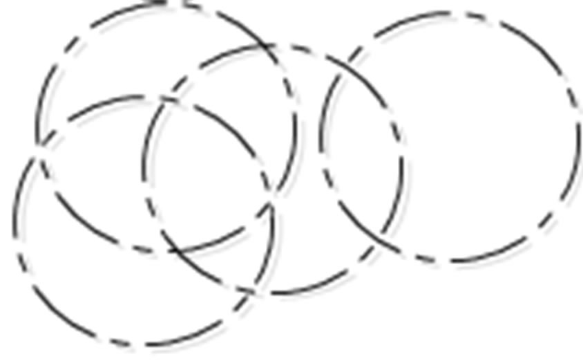
Two sensors creates three regions if they overlapped see Figure 1. The function 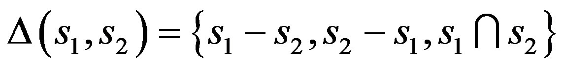 is expressing the created regions. For convenient, we will express the created regions by
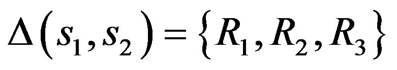 . The symbol
  denotes to the number of created regions. For example
 . Each region of
  has a coverage degree. The symbol
  denotes the coverage degree.
The symbol 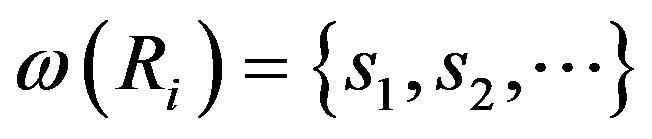 denotes the set of sensors covered the
  region.
 .
.
A group of k sensors
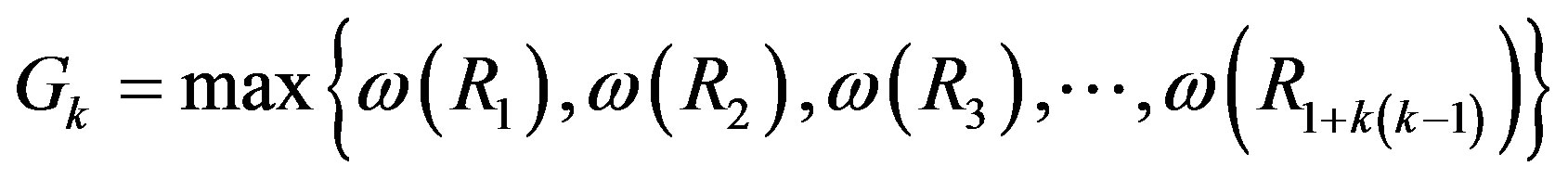 .
.
For example,
 .
.
In [16], the authors provided an analysis about grouping strategy of WSN. We will used this idea to divide the WSN into groups and then organize these groups in order to facilitate the routing process. This grouping scheme is not useful if the sensors moving quickly.
3. Sensors Grouping Algorithm
In this section, we will provide recursive algorithm to divide the overloaded sensors in to separated groups. A deep explanation is provided in Appendix. We will start by define the terms to be used in our algorithm.
3.1. Definitions
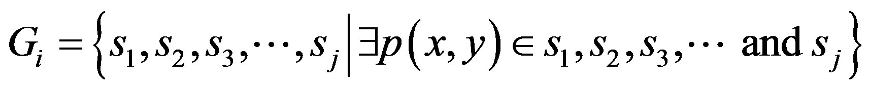
Group of Sensors : is a set of sensors that are overlapped while covering the same region in the sensing field.
In the this paper, we will use the notation  to
to
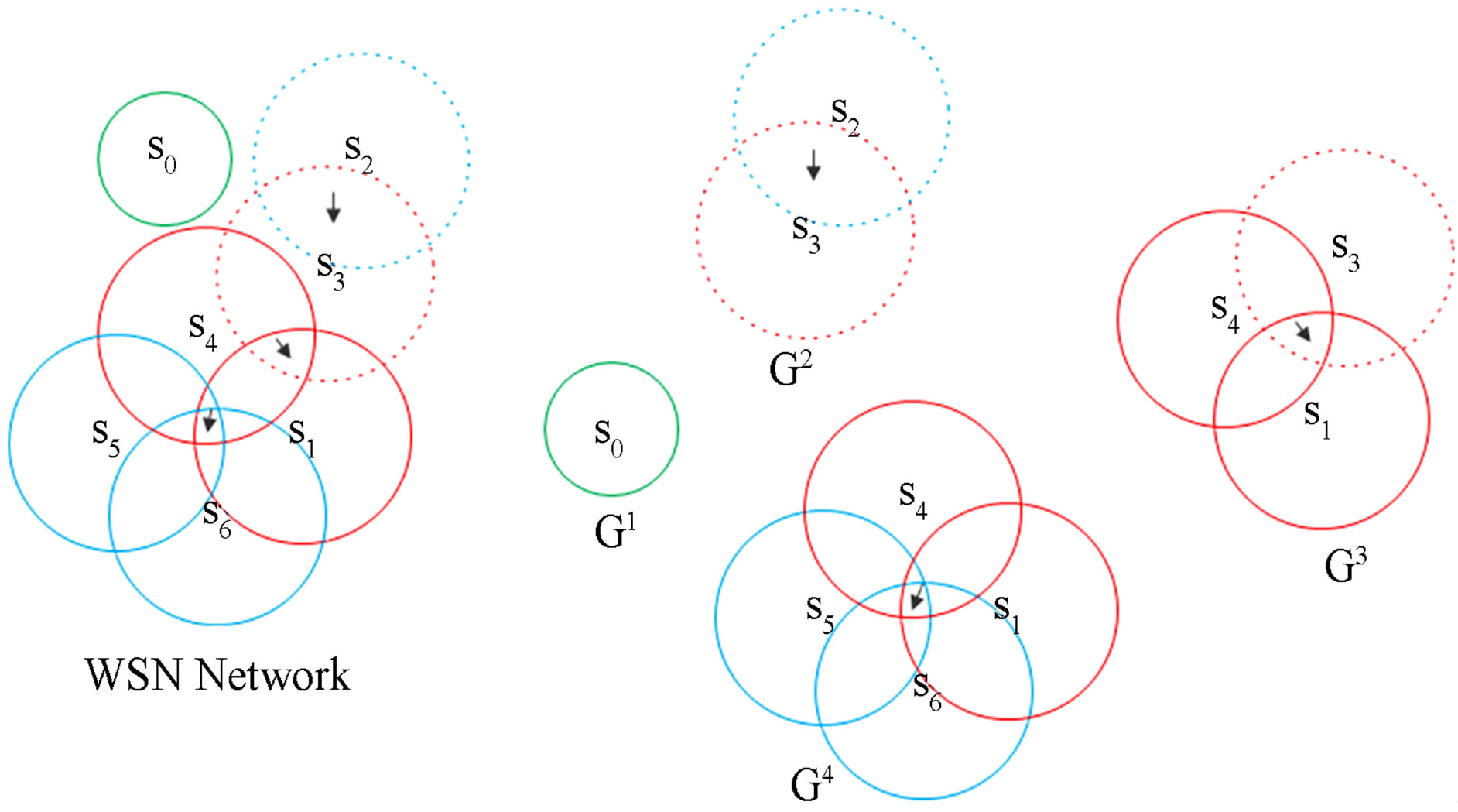
Figure 1. Partition the WSN into sensors’ group.
indicate the sensor  overlapped with sensor
 . More precisely,
  covered the same region. The group of sensors is an object containing the members shown below.
ClassSensorGroup
{
intGroupID { get; set; }
intGroupLength { get; set; }
stringGroupMembersString { get; set; }
stringGroupingMethod { get; set; }
List
}
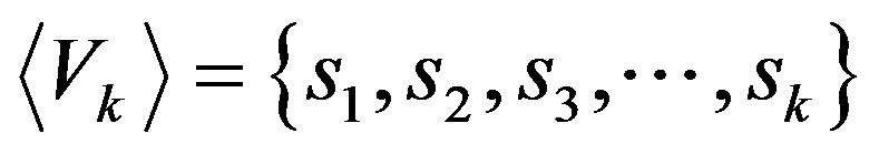
Vector of a Sensor : is a set of sensors, which are overlapped with the sensor si.
Each sensor in the network has a vector. Some of the sensors inside the network have the same vector. The vector is an object:
class Vector
{
intSensorID { get; set; }
int Length { get; set; }
stringSensorsOverlappingString { get; set; }
List
Ellipse SensorBody{ get; set; }
Sensor Sensor{ get; set; }
}
Direct Group : is a group of sensors that fully matches a vector in the network.
Indirect Group : is a Hybrid and collected group of sensors by processing multiple vectors.
Matched Direct Groups of a Vector: The sensors in ungrouped vectors  are not fully matched with any direct group
 , but they can matched some sensors in multiple direct groups, some sensors of ungrouped vectors might not be matched with any sensors in the directed groups.
Suppose an ungrouped vector:
 A list of direct groups:
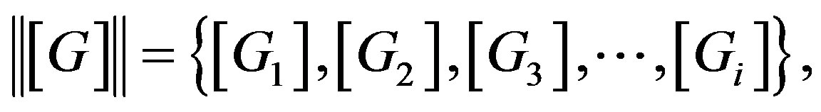
Each group contain a number of sensors
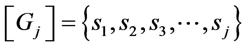 .
.
The matched group:
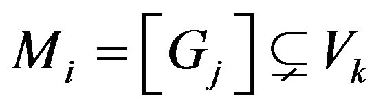
Remnant Sensors: remnant sensors  are those sensors in ungrouped vectors
  that do not matches any sensor in direct group.
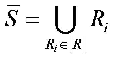
Solid Vector: The solid vector  is the union of remnant sensors
  of each ungrouped vectors.
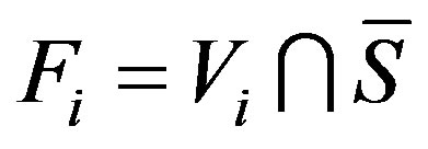
Filtered Vectors: By finding the solid vector , we can exclude all the sensors directly grouped already and also find the sensors that are not grouped yet. For each ungrouped vector
 ,
,
3.2. System Model
The wireless sensor network is a list of vectors collected by all sensors in the field. The network of n sensors is represented by a square matrix .
.
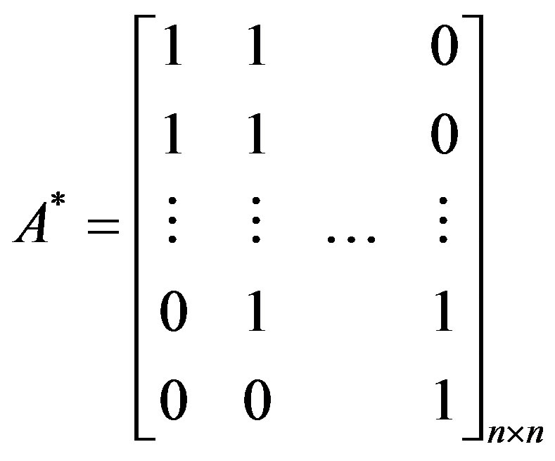
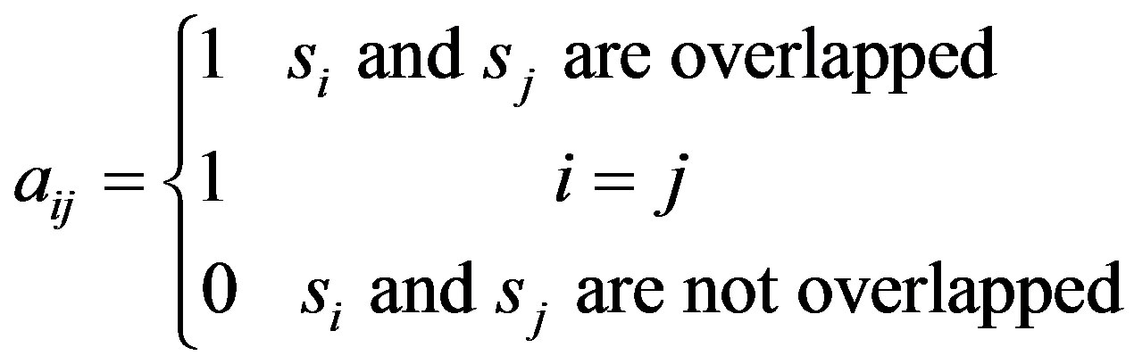
To facilitate the calculations, assume that the numerical value of sensors in the matrix is either 1 or 0 as below.
We can find the maximum coverage degree areas by partitioning  into square sub-matrices
  , such as the value of each sensor of sub-matrix
  as well as the sub-matrix contain the maximum possible number of rows and columns. Each sub-matrix should match a group of sensors. For example, the network in Figure 2 is partitioned into five square sub-matrices shown as below.
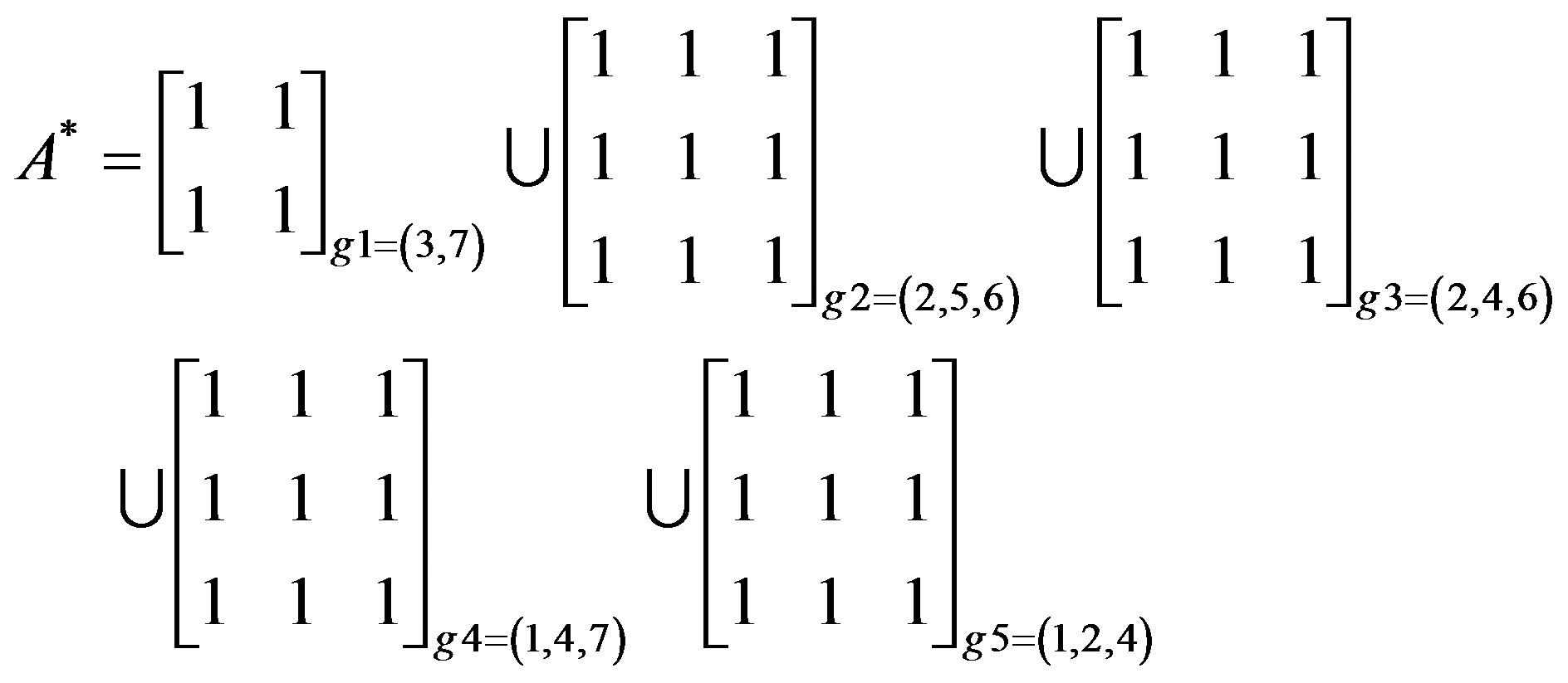
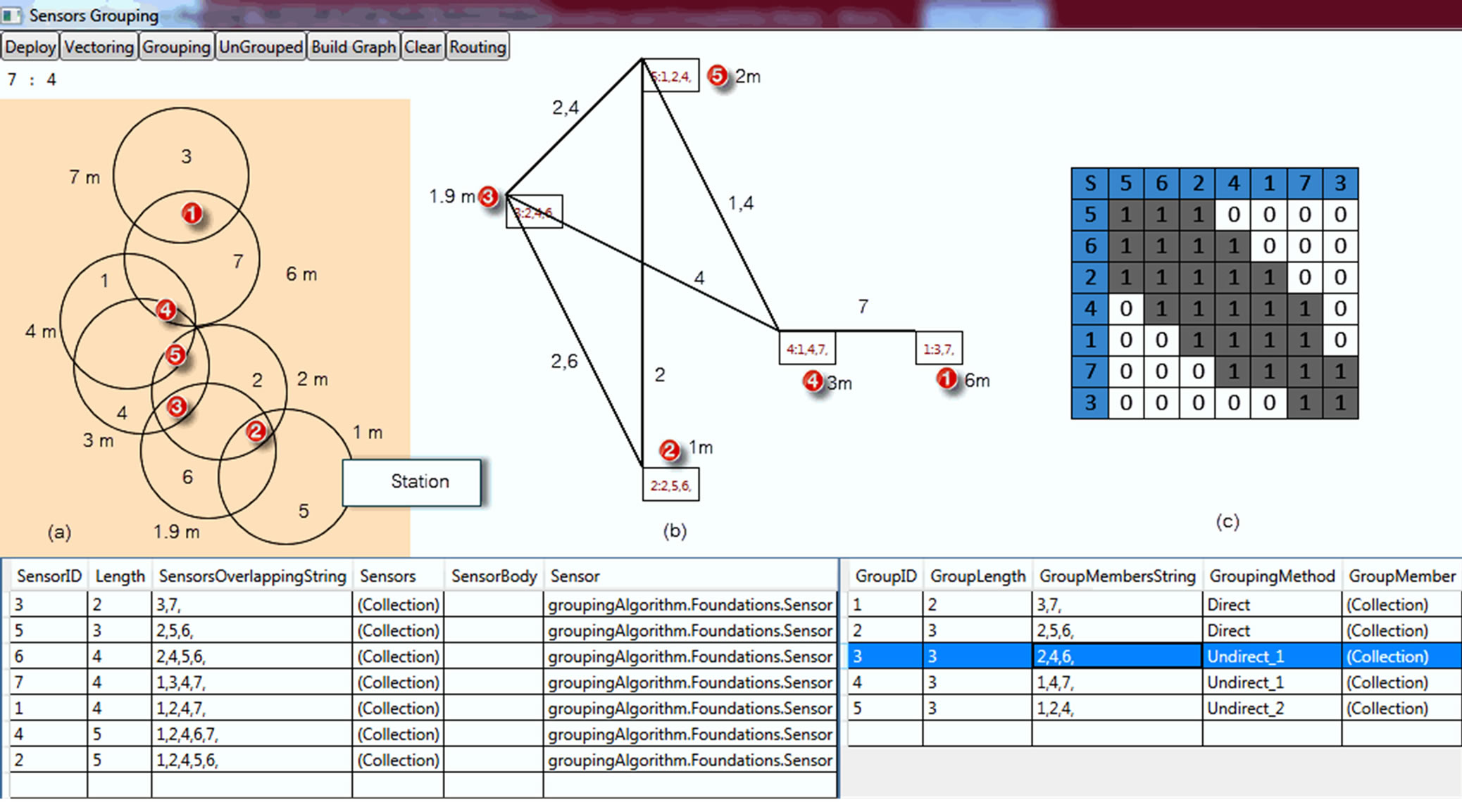
Figure 2. Implementation of the grouping algorithm graph. (a) Sensing field; (b) grouping graph; (c) grouping matrix.
We can see that each group of overlapped sensors is a square matrix, and the value of each element of the matrices is 1. Simply, we just find out the square matrices with the following conditions: The maximum possible number of rows and columns should be alighted together and the value of each element is 1. Suppose that each sensor  in the field sends a vector
 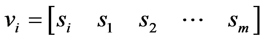 to the base station, all vectors create the
 . Let
. Let  be the number of sensors of
 . In addition to that, let R be the number of repetition of
  in
in . The first step of this algorithm is to find the sensors overlapping relations based on their distance; each sensor has a vector of sensors. The second step is to sort these vectors according to the number of sensors within.
3.3. Groups Algorithm
Finding a group of sensors indirectly can be manipulated by dividing ungrouped vectors into smaller vectors so that the sensors that are directly grouped already are not needed. To do so, we can follow the steps below:
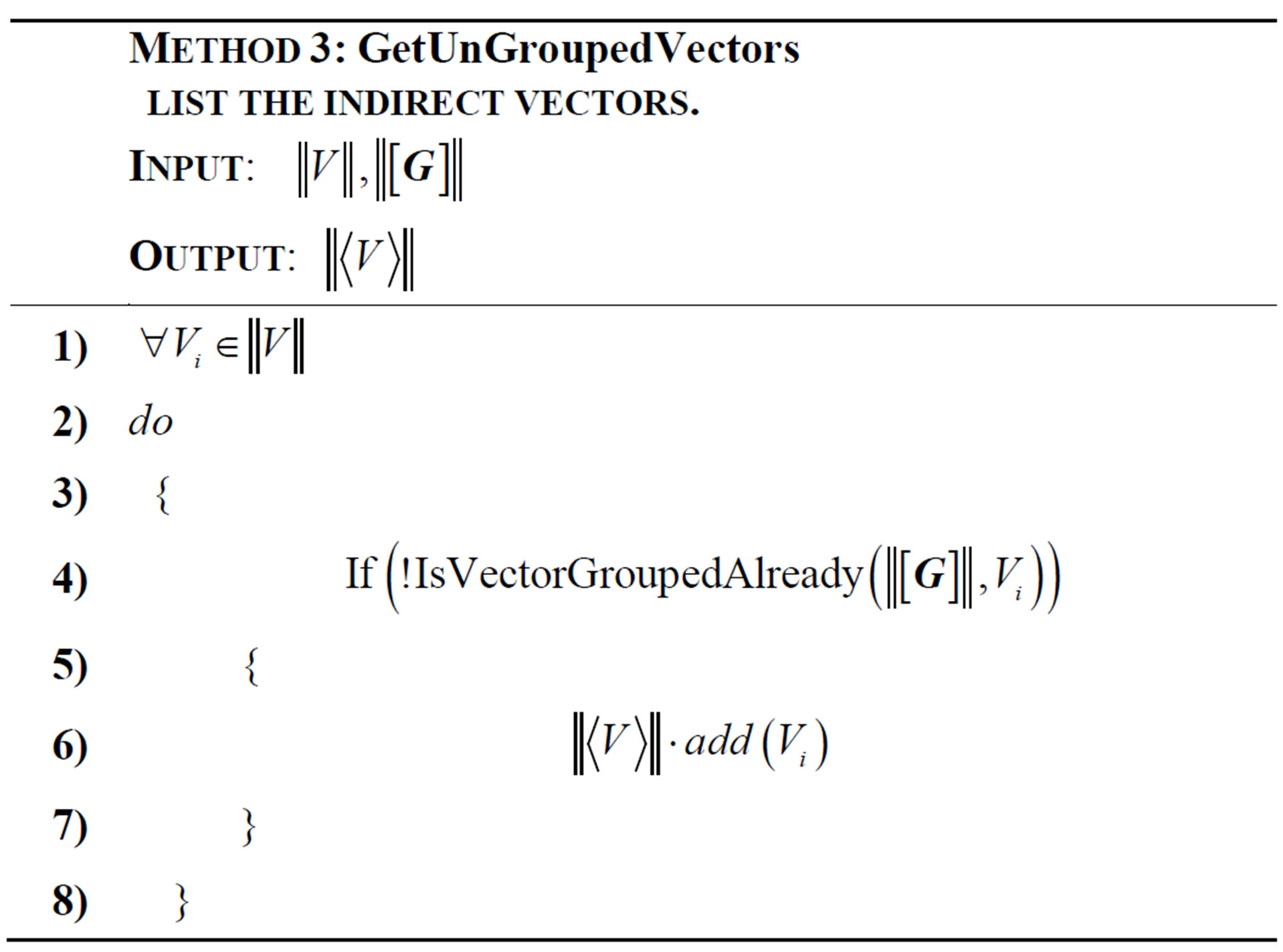
1) Find ungrouped vectors by comparing the direct groups and the network vectors list (GetUnGroupedVectors ).
).
2) Find the matching direct groups associated to ungrouped vectors (GetMatchingGroupsForVector
 ).
).
3) Find the solid vector, which contains the remnant sensors of ungrouped vectors list (GetSolidVector
 ).
).
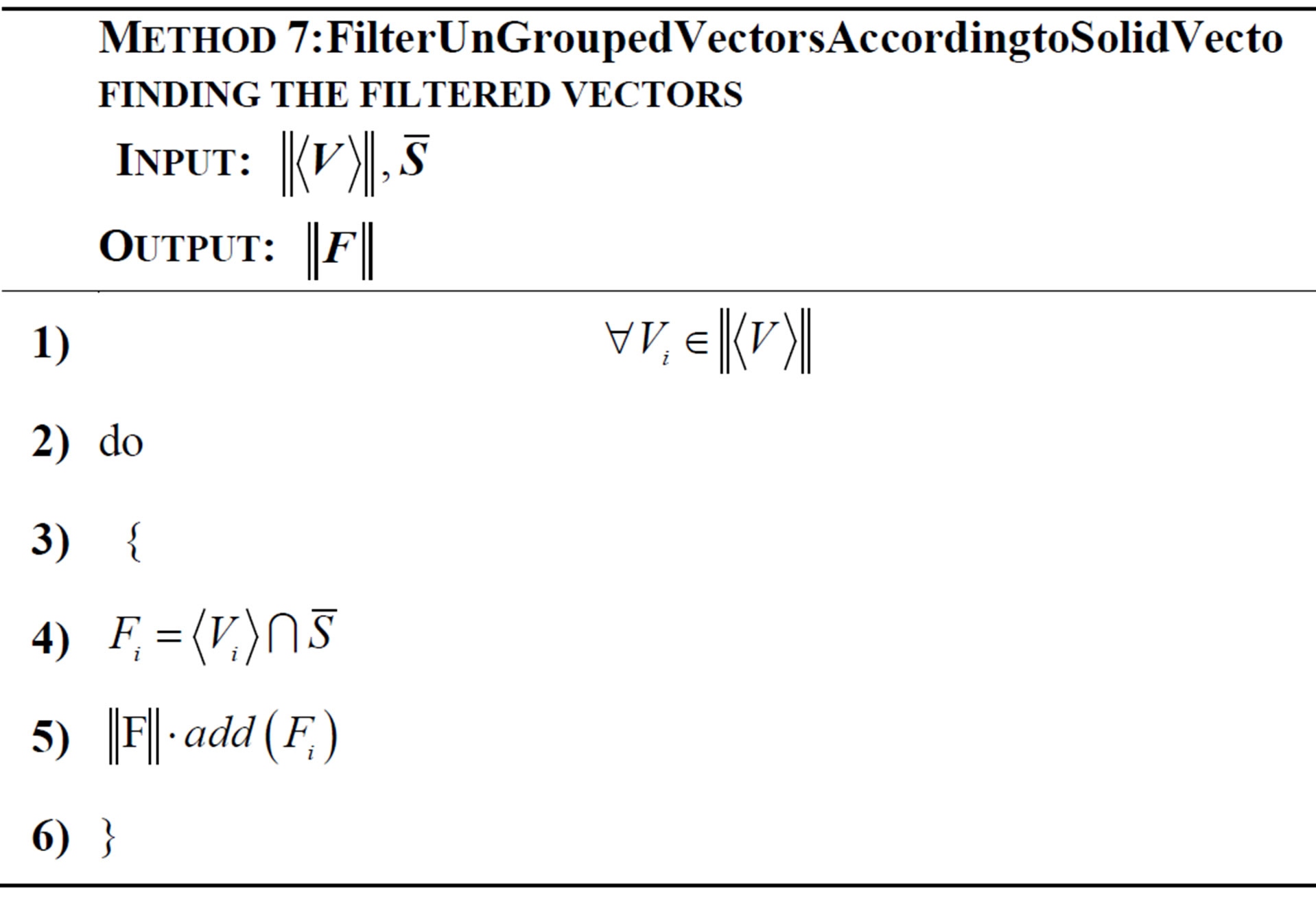
4) Filter ungrouped vectors according to the solid vector (FilterUnGroupedVectorsAccordingtoSolidVector
 ).
).
5) Extract new groups from filtered ungrouped vectors  by calling the method of finding the direct groups (GetDirectGroups
 ).
).
6) Repeat the steps from step 1 to step 5 recursively until no new groups are found (Algorithm 1).
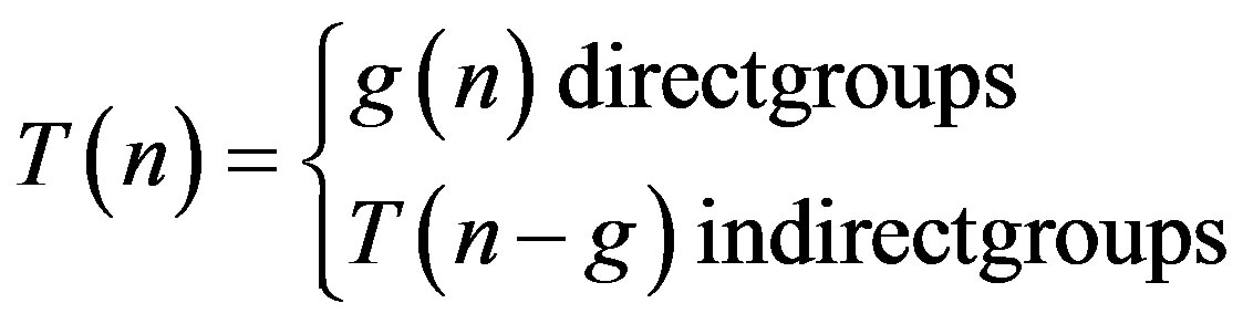
Recursive algorithms solve the problem by solving smaller versions of the same. The smaller versions of ungrouped vectors are about half the size of the original vectors. The algorithm can be referred to as a “divide and conquer” algorithm. Say that we have (n) of original vectors, the time needed to extract (g) direct groups is . However, not all vectors are able to be directly grouped. For ungrouped vectors, there will be (n-g) vectors. The recursive time needed is:
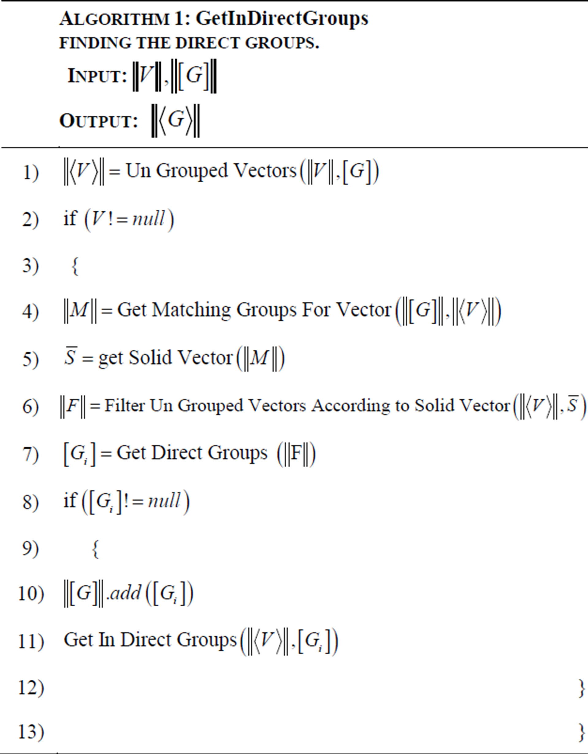
Algorithm 1. Finding the direct groups.
The analysis depends on the preparation work to divide the input, the size of the ungrouped vectors, the number of recursive calls and the concluding work to combine the results of the recursive calls.
g is the number of extracted groups of each recursive call.
4. Routing Basing on Group of Sensors
4.1. Sensors Graph
The routing algorithm is started by dividing the wireless sensors network to independent groups (explained in Subsection 3.3). Each group is comprised of a certain number of sensors. A Sensor may belong to more than one group. If a sensor belongs to group A and belongs to group B, we say there is a link between group A and B, and we call this sensor by coordinator or the group leader. Each group contains one or more leaders.
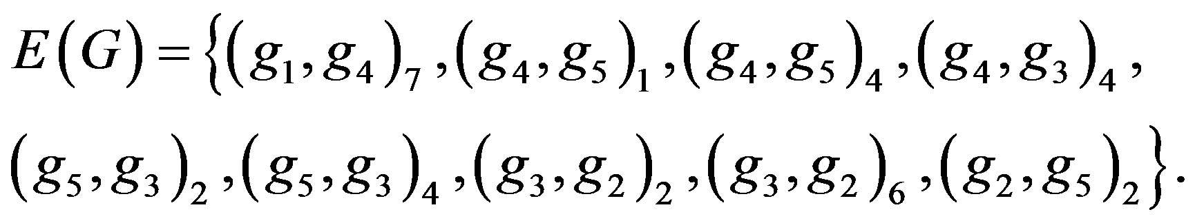
The graph of sensor network  consists of a finite nonempty set V of groups called vertices and a set E of 2-elements of V called edges. In the graph theory, the notation V(G) is the set of vertex and E(G) is a set of edges. Using the idea of graph theory, we can say that each vertex is represented by a group of sensors. The leader of the group is represented with an edge. As long as the graph is connected, there will be a path from the source node connecting the base station, hence the packet must be reaching the sink node. Here we assume that connectivity and coverage of network are managed well.
The graph in Figure 2 can be represented mathematically by
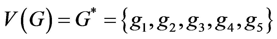 ,
,
The degree d(v) of a vertex V is its number of incident edges. Any two groups have an incident edges called to be neighbor groups. Each group has at least one neighbor otherwise the network is disconnected. Let 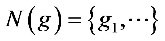 is the neighbor groups of g for instance in Figure 2,
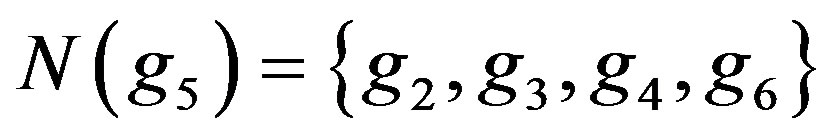 .
.
The distance between the source node and the sink node is an important parameter to control and improve the performance of packet forwarding in the overall network. Considering the power consumption, the nearest nodes to the sink could save more power by building a shorter path with a minimum number of hops. Since our algorithm is based on grouping, we need to define the term of grouping distance, the distance of group is the least distance among sensors inside the group to the base station. Should we denote to the distance between sensor s1 and the base station by . In Figure 2,
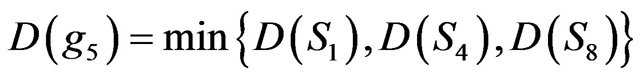 .
.
We assumed each that group is taking into account the information of its neighbor groups’ distance. With adaptive routing, when a source group has to forward a packet towards a particular group, it can choose the leader sensor to use from a set of alternative leaders associated to the group. This selection can be done upon two conditions: the first condition is the current state of the leader (busy or free) and therefore, the busy leaders are skipped. The second condition is the least distance to the base station and therefore, the nearest group to base station can be selected.
4.2. Finding Leaders
The Leader sensor acts as direct link among its associated groups. It can keep forwarding the data packet to all groups it belongs to. Straightforwardly, we can list the leaders by the simple algorithm below (Algorithm 2).
4.3. Selecting the Leader
Each group has a set of neighbors and a set of leaders. When a packet has been forwarded to a group, the group should know well its leaders and neighbors and therefore make the decision of packet routing to the next hop. In Output: Leaders Find
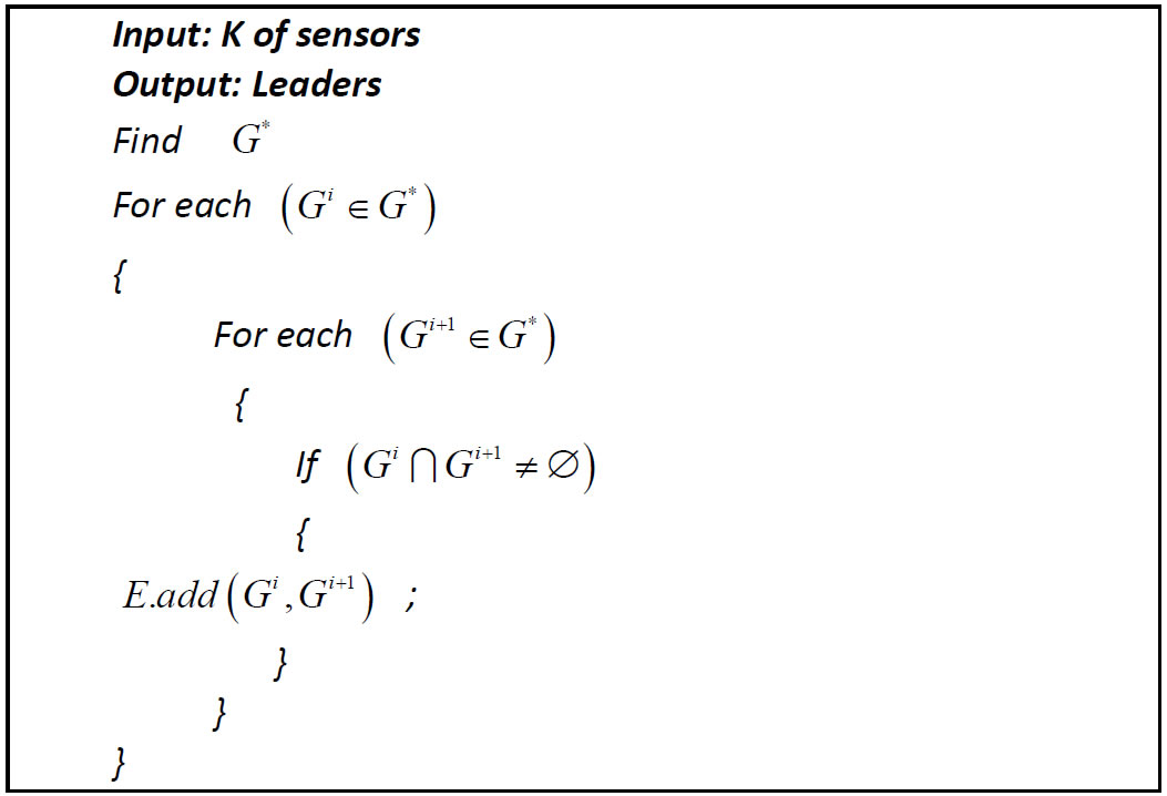
Algorithm 2. Finding the leaders.
the source group, there are one or more leaders connecting to one or more neighbors.
Multiple leaders in the source node might link a single neighbor. In addition, the leader might connect to multiple neighbors. Thus, after selecting the nearest neighbor group, we must ensure that the connecting leader is free, otherwise, the packet cannot be forwarded via this leader. If the leader is busy, then the packet must be forwarded to the second nearest neighbor. If there is only one leader in the source node, the packet should be delayed until the leader becomes free.
The selection process of the leader is running simply by choosing the nearest neighbor and checking the availability of the leader connected to this neighbor. If the leader is free, then this is the adaptive channel to forward the data. There will be more than one adaptive channel when there are more than one leaders (parallel leaders) connected to nearest neighbor. If the current state of all parallel leaders is busy, then there will be two ways to deal with: the first way, the packet should wait until one of the parallel leaders becomes free. However, this is not respectable in case the application’s demand is a real time stream of monitoring. The second way: if the source node contains other leaders connecting to other neighbors, the packet can be forwarded to any other neighbor. However, this might lead to an increment of the number of routing hops, hence might maximize the usage of energy in the overall network, this might lead to the death of a sensor. If there is only one neighbor associated to the group and all leaders are busy, then the first way is obligatory. In case of all parallel leaders are free, any leader election algorithm can be applied to manage the selection of the leader.
Leaders in the same group are called partners. Moreover, if more than one leader is connected to the same neighbor group, they are called twin leaders. A set of leaders in a group can be partners or twins, neighbors can determine this. For example, in Figure 2, group 5 contains three elements, three of them are leaders, and thus leaders 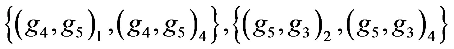 are twins. If a leader connected to more than one neighborgroup is called identical leader, for example,
  and
and  are identical Leaders.
In Method 1, the input is the source node (SensorGroupSourceGroup), and a list of neighbors associated to the source node (List
4.4. Numerical Example
As shown in Figure 2, (a) sensors are deployed in the field. Say, sensor (3) detects a target. Here we assume that all leaders are free. The packet routing from sensor (3) to the station is going according to the steps below (see Figure 3). The source groups (G1) have one neighbor and one leader, forwarding data towards group (G4) via sensor (7) obligatory. When the packets arrived to (G4), it has four leaders and three neighbors, the min group distance is to (G3), hence the next hop is (G3) via sensor (4). After the packet has arrived to (G3), this Input: a group of sensors, and a list of Neighbor groups.
Output: a sensor called leader.
Sensor SelectLeaderSensor(SensorGroup SourceGroup ,List
{
Sensor Leader = null;
Neighborgroups SelectedNeighbor = SelectMinDistanceNeighbor(Neighbors);
List
LeaderAssociatedwithNeighbor(SourceGroup, SelectedNeighbor);
Sensor selectFreeSensor =
SelectFreeSensor(LeadersAssociatedwithSelectedNeighbor);
Leader = selectFreeSensor;
return Leader;
}
Method 1. Select leader.
Output: Forward packet Find
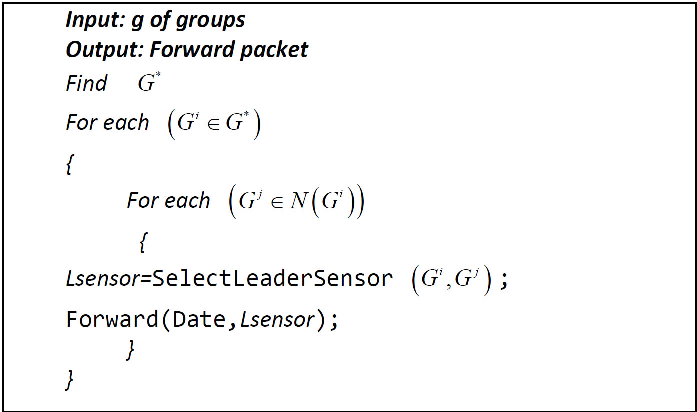
Algorithm 3. Routing basing on groups.
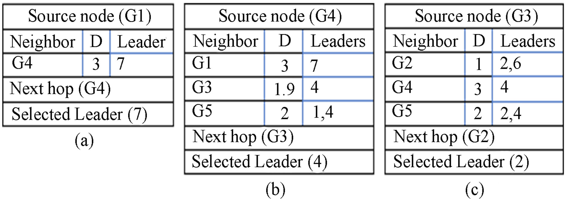
Figure 3. Routing tables in each source node from (G1 to G2) when all sensors are free.
group (5) leaders and three neighbors, the min group distance is to (G2), Thus, the next hop is (G2) via sensor (2).
5. Performance Evaluation
In this section, we will evaluate the impact on network performance of the proposed routing algorithm. For this purpose, we have developed a detailed simulator that allows us to estimate the network performance, power consumption, and the number of hops. The results are shown in the Figures 4-6.
Counting the Average Number of Hops
The number of hops depends on the number of groups. Say we have n nodes deployed randomly in the sensing field, and want to compute the number of possible groups that can be generated. A pattern of groups is a deployment way for sensors groups such that all sensors in the group are connected. Let’s start by a simple example with n = 4. As shown in Table 1 and Figure 7, there are four grouping patterns.
Let us denote to the pattern by  and to the number of hops of each pattern by
 .
.
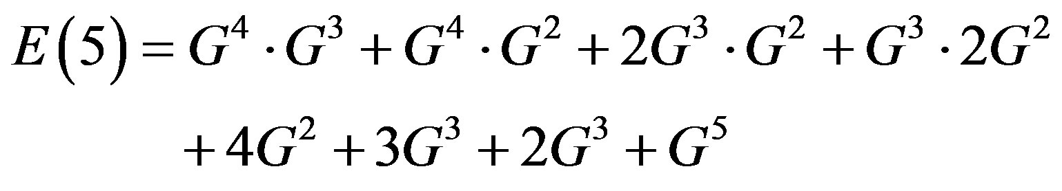
The expression of patterns can be written as:
Easily we can see the patterns of four sensors are:
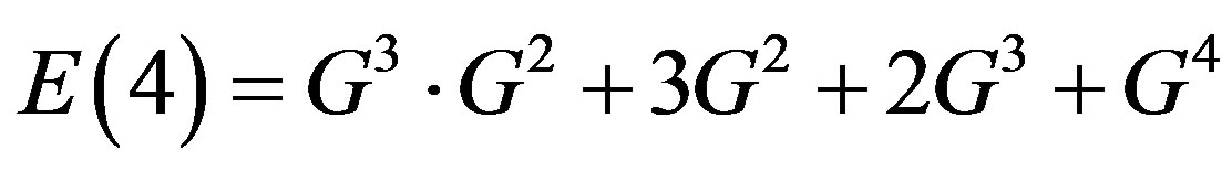
For five sensors, there will be eight patterns.
Let us donate to the number of pattern by . For n sensors, there will be
 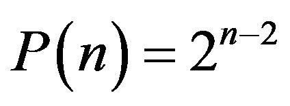 patterns.
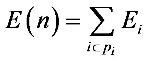
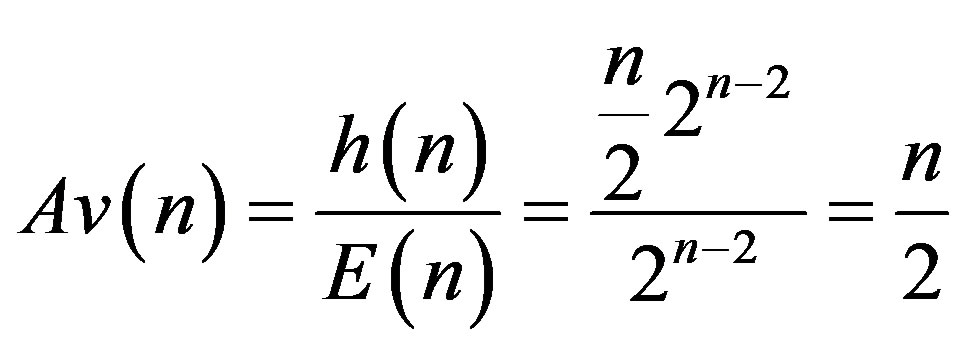
The number of hops is changed according to patterns. Let  be the sum of hops of all patterns. For example,
 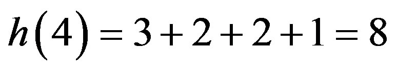 as shown in Table 1 and Figure 7, it is easy to find that the average number of hops is
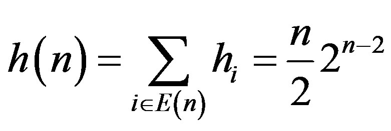
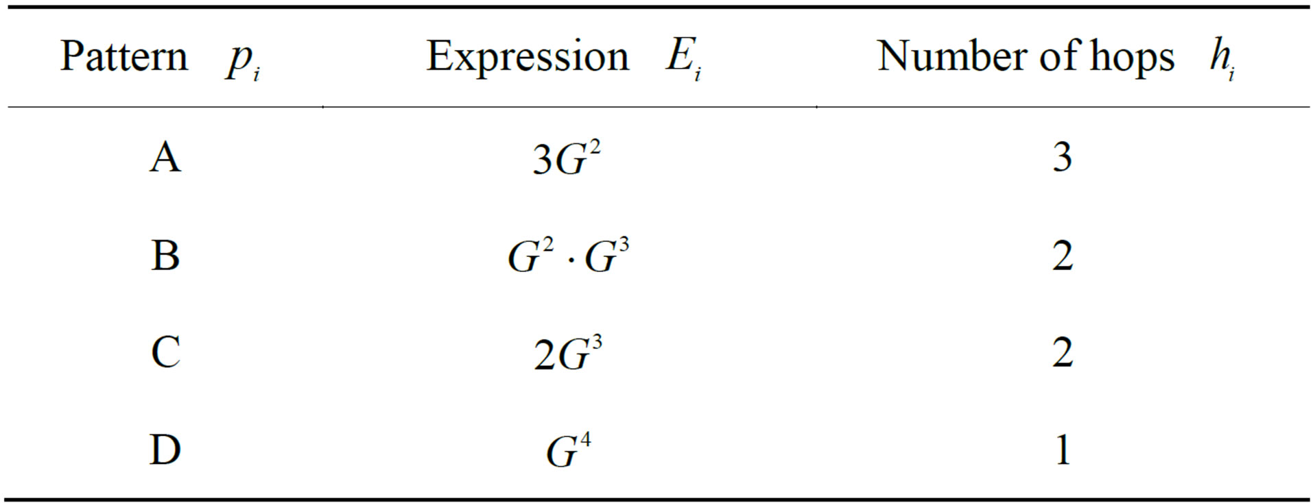
Table 1. Grouping patterns of four sensors deployed (see Figure 7).
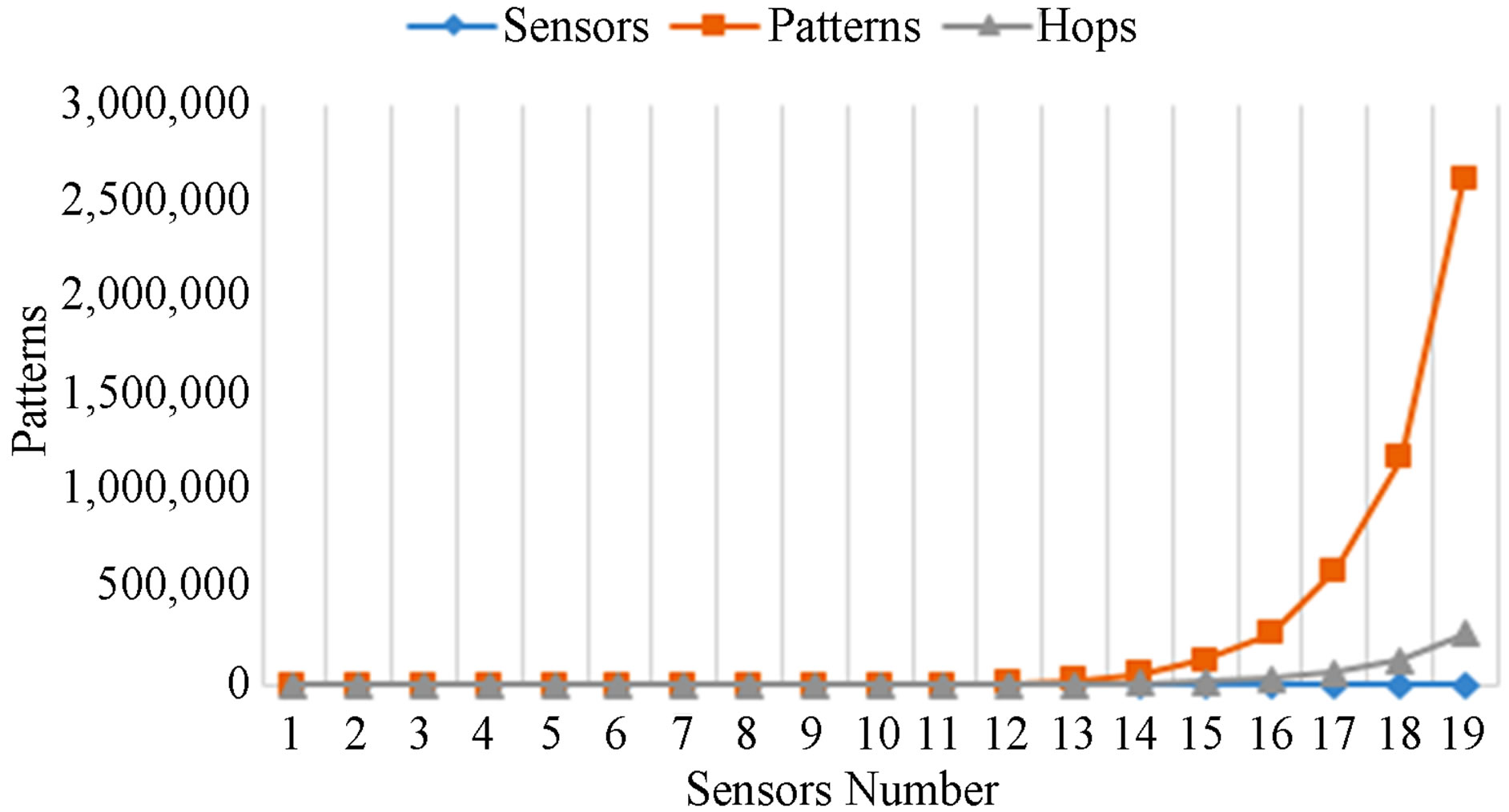
Figure 4. Pattern count and hops.
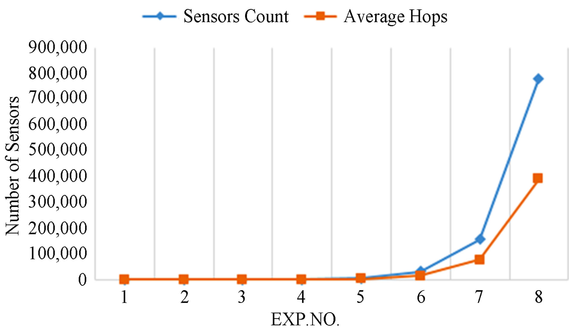
Figure 5. Evaluation of average routing performance based on the grouping algorithm.
In the second experiment, there are 10,000 nodes deployed in different coverage degree. Say we have N sensors deployed randomly. Let us say that the degree of network coverage is C, the complexity of algorithm (See Figure 6).
6. Conclusion
We have proposed an algorithm where the source group forwards a packet to one neighbor only and there is no need of flooding or forwarding packets to all neighbors. The grouping adaptive routing saves more power therefore, ends up maximizing the lifetime of the wireless sensor network.
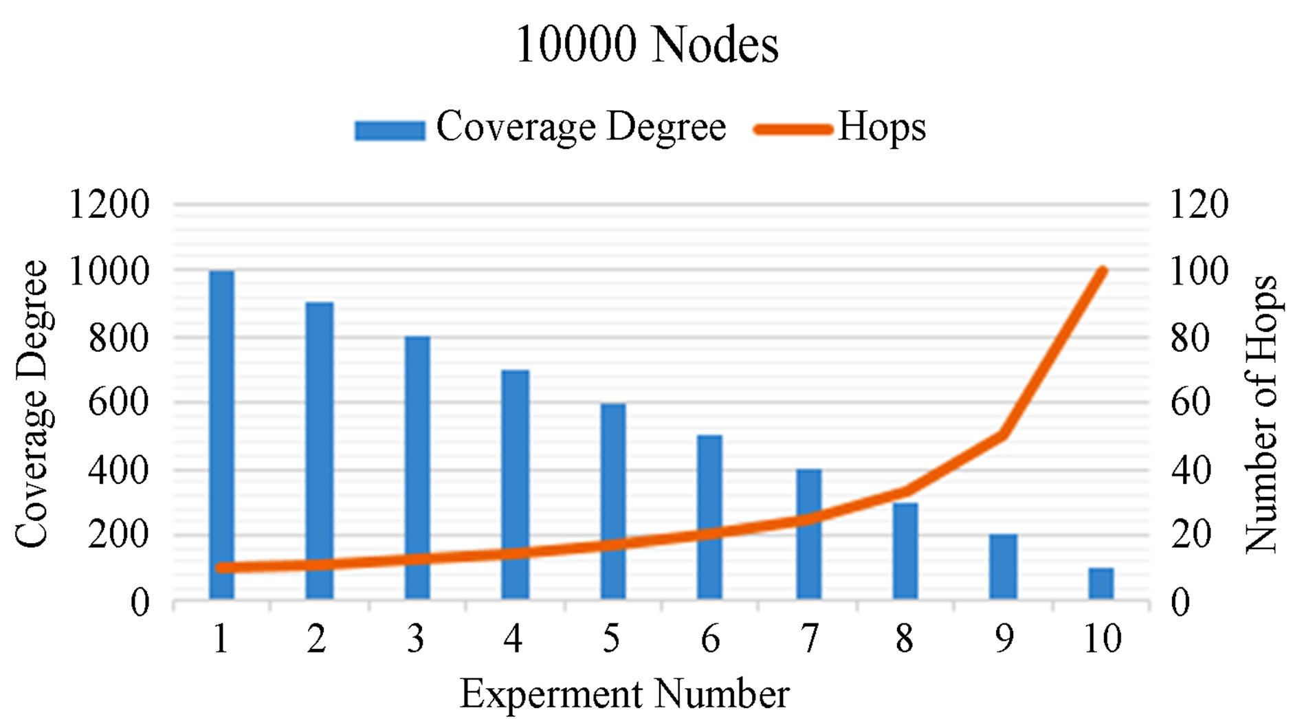
Figure 6. Evaluation of routing performance based on the grouping algorithm on different coverage degrees.
 (a)
(a)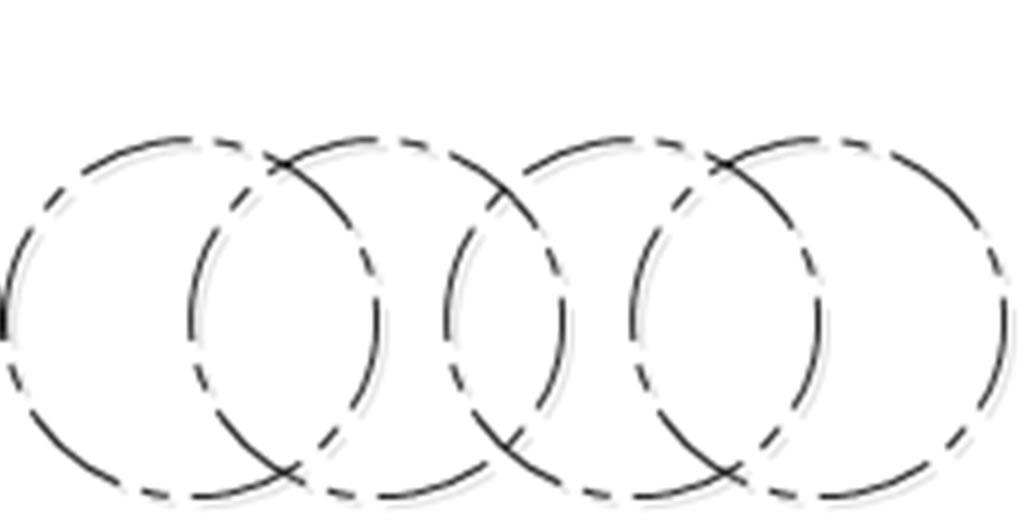 (b)
(b)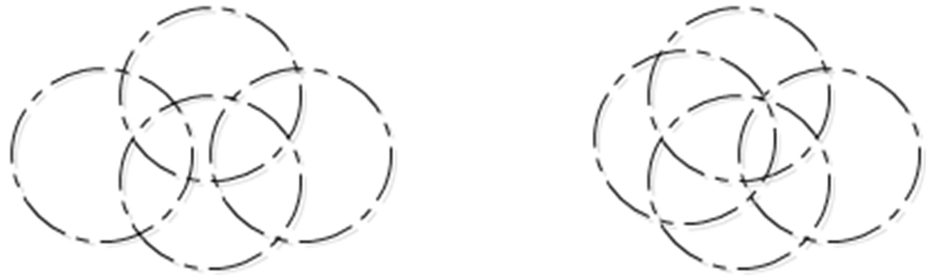 (c)
(c)
Figure 7. Grouping patterns of four sensors deployed.
Acknowledgements
The authors would like to acknowledge The National Natural Science Foundation of China, the National Science Technology Major Project and the China Scholarship Council for their supports.
REFERENCES
- L. J. G. Villalba, A. L. S. Orozco, A. T. Cabrera and C. J. B. Abbas, “Routing Protocols in Wireless Sensor Networks,” Sensors, Vol. 9, No. 11, 2009, pp. 8399-8421.
- E. Zanaj, M. Baldi and F. Chiaraluce, “Efficiency of the Gossip Algorithm for Wireless Sensor Networks,” In Proceedings of the 15th International Conference on Software, Telecommunications and Computer Networks (SoftCOM), Split-Dubrovnik, September 2007.
- J. C. Martinez, J. Flich, A. Robels, P. Lopez and J. Duato, “Supporting Adaptive Routing in infiniband Networks,” Proceedings of the 11th Eromicro Conference on Parallel, Distributed and Network-Based Processing (Euro-pdp03) 2003.
- S. C.-H. Huang, S. Y. Chang, H.-C. Wu and P.-J. Wan, “Analysis and Design of Novel Randomized Broadcast Algorithm for Scalable Wireless Networks in the Interference Channels,” IEEE Transactions on Wireless Communications, Vol. 9, No. 7, 2010, pp. 2206-2215.
- H. H. Zhang and J. C. Hou, “Maximising α-Lifetime for Wireless Sensor Networks,” 2007.
- M. Cardei and D. Z. Du, “Improving Wireless Sensor Network Lifetime through Power Aware Organization,” Wireless Networks, Vol. 11, No. 3, 2005, pp. 333-340.
- S. Poduri and G. Sukhatme, “Constrained Coverage for Mobile Sensor Networks,” IEEE International Conference on Robotics and Automation, New Orleans, April 26-May 1, 2004, pp. 165-172.
- A. Chen, S. Kumar, and T.-H. Lai, “Designing Localized Algorithms for BarrierCoverage,” MOBICOM. ACM, 2007.
- X. Bai, Z. Yun, D. Xuan, T. Lai and W. Jia, “Optimal Patterns for Four-Connectivity and Full Coverage in Wireless Sensor Networks,” IEEE Transactions on Mobile Computing, 2008.
- J. Wu and S. Yang, “Coverage and Connectivity in Sensor Networks with Adjustable Ranges,” International Workshop on Mobile and Wireless Networking (MWN), 2004.
- M. Cardei, J. Wu, N. Lu and M. O. Pervaiz, “Maximum Network Lifetime with Adjustable Range,” IEEE Intl. Conf. on Wireless and Mobile Computing, Networking and Communications (WiMob’05), 2005.
- M. Cardei, M. T. Thai, Y. Li and W. Wu, “Energy-Efficient Target Coverage in Wireless Sensor Networks,” Proceedings of IEEE Infocom, 2005.
- M. Cardei and D.-Z. Du, “Improving Wireless Sensor Network Lifetime through Power Aware Organization,” Wireless Networks, Vol. 11, No. 3, 2005, pp. 333-340.
- J. K. Hart and K. Martinez, “Environmental Sensor Networks: A Revolution in the Earth System Science?” Earth-Science Reviews, Vol. 78, No. 3, 2006, pp. 177-191.
- Y. Ma, M. Richards, M. Ghanem and Y. Guo, “Air Pollution Monitoring and Mining Based on Hassard Sensor Grid in London,” Sensors, Vol. 8, No. 6, 2008, p. 3601.
- H. Ammar, X. F. Wang and Y. Xiong “Sensors Grouping Model for Wireless Sensor Network,” Journal of Sensor Technology, Vol. 3, No. 4, 2013, pp. 133-140.
Appendix
Listing of Vectors
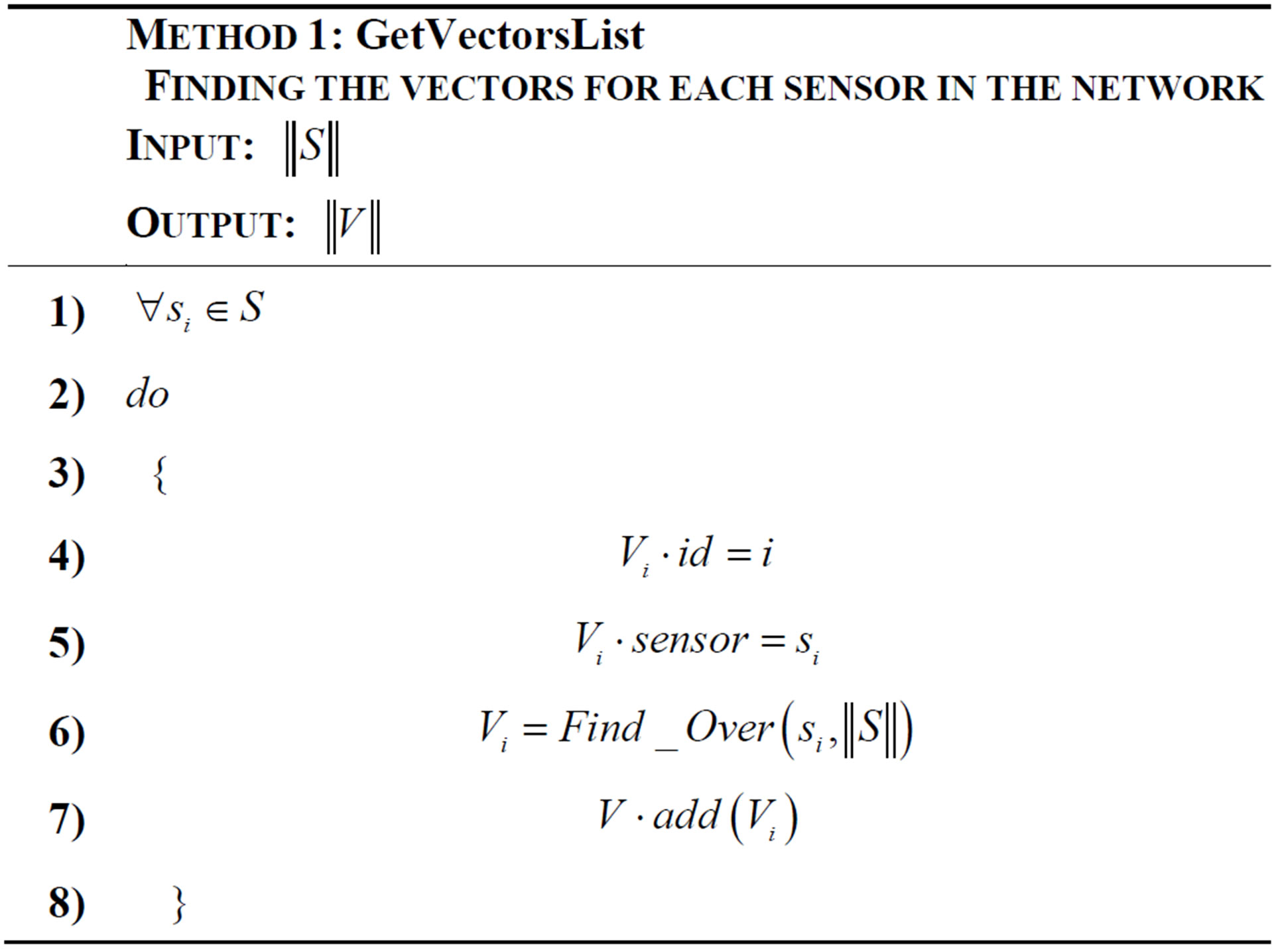
According to Method 1, GetVectorsList, the input  is a list of sensors deployed in the sensing field. The output
  is a list of vectors. The main procedure here is to find the overlapped sensors with the required sensor
 . Each sensor si finds the overlapping list of sensors and sends it to the base station where the square matrix of network A* is built. The algorithm for finding the groups will run in the base station. In case the grouping process run internally in the local node, each node send its vector to the adjacent node only. Here we suppose the grouping process will run externally.
Direct Grouping
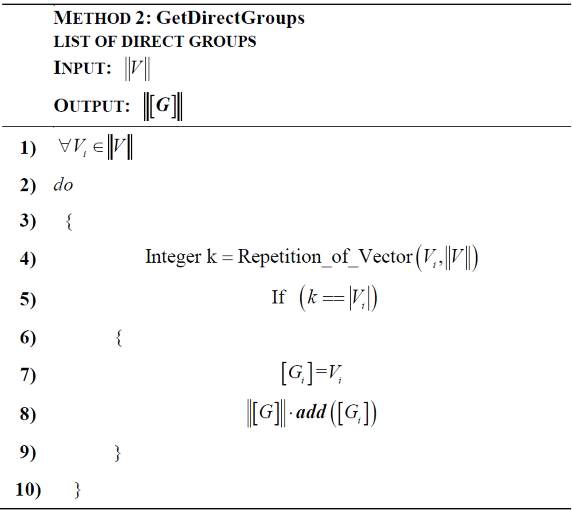
In the Method 2, GetDirectGroups, the input of algorithm  is a list of vectors of all sensors deployed in the field. The output
  is a list of direct groups extracted from the list of vectors.
Ungrouped Vectors
For each vector  in the network list
 , if not matched any entry
  in the direct groups list
 , then it considered as ungrouped vector
 .
.
 .
.
In the Method 3, GetUnGroupedVectors, the inputs are  a list of the network vectors and the direct groups
 . Therefore, we just find those vectors, which are not grouped yet.
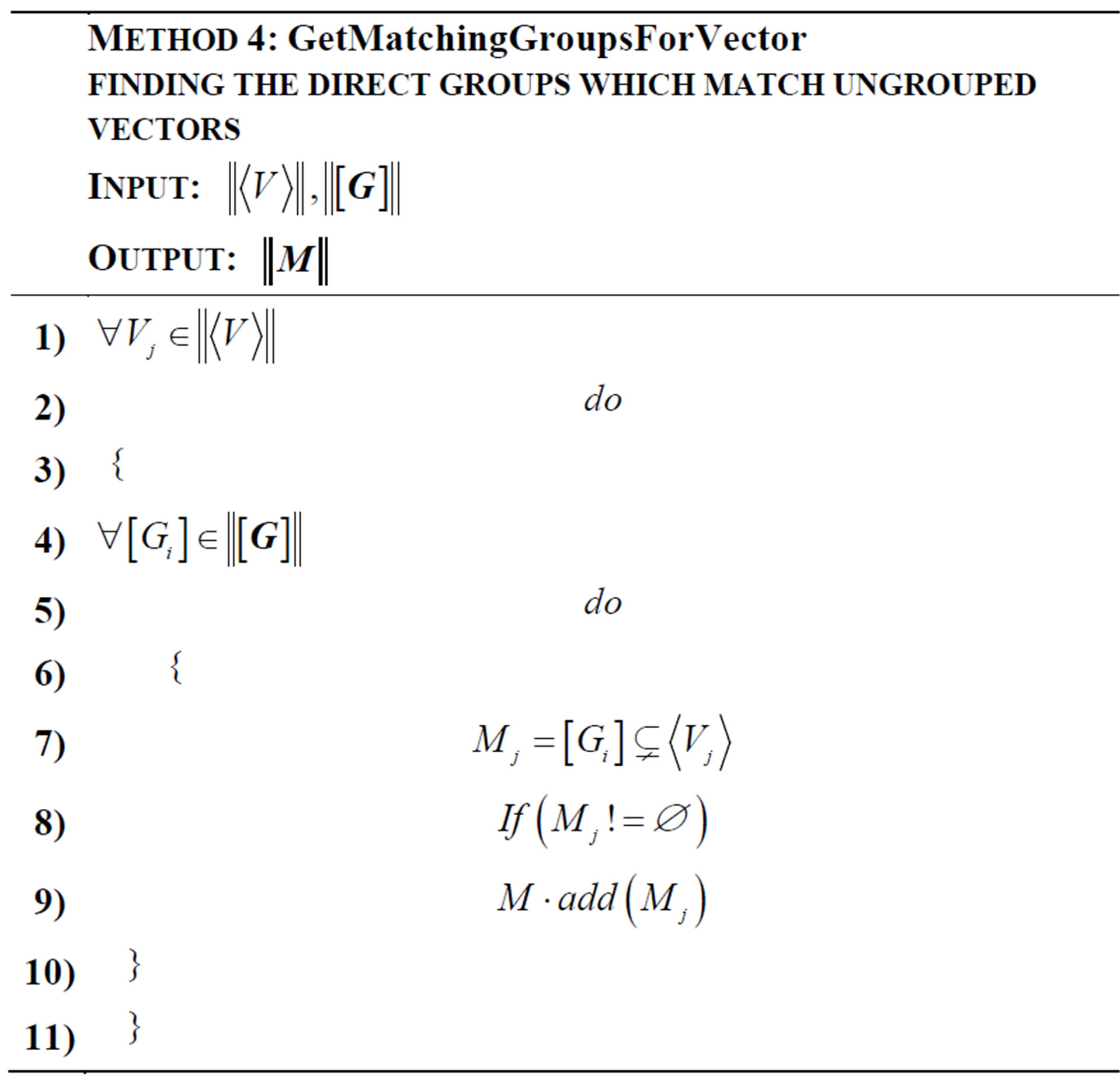
Finding the Matching Direct Groups of a Vector
In the Method 4, GetMatchingGroupsForVector, the input  is a list of direct groups and
  is a list of ungrouped vectors. The output
  is a list of the direct groups which matched the ungrouped vectors. For each ungrouped vector, we will find the matching direct groups by dividing the ungrouped vectors into smaller vectors. Each ungrouped vector might match multiple direct groups.
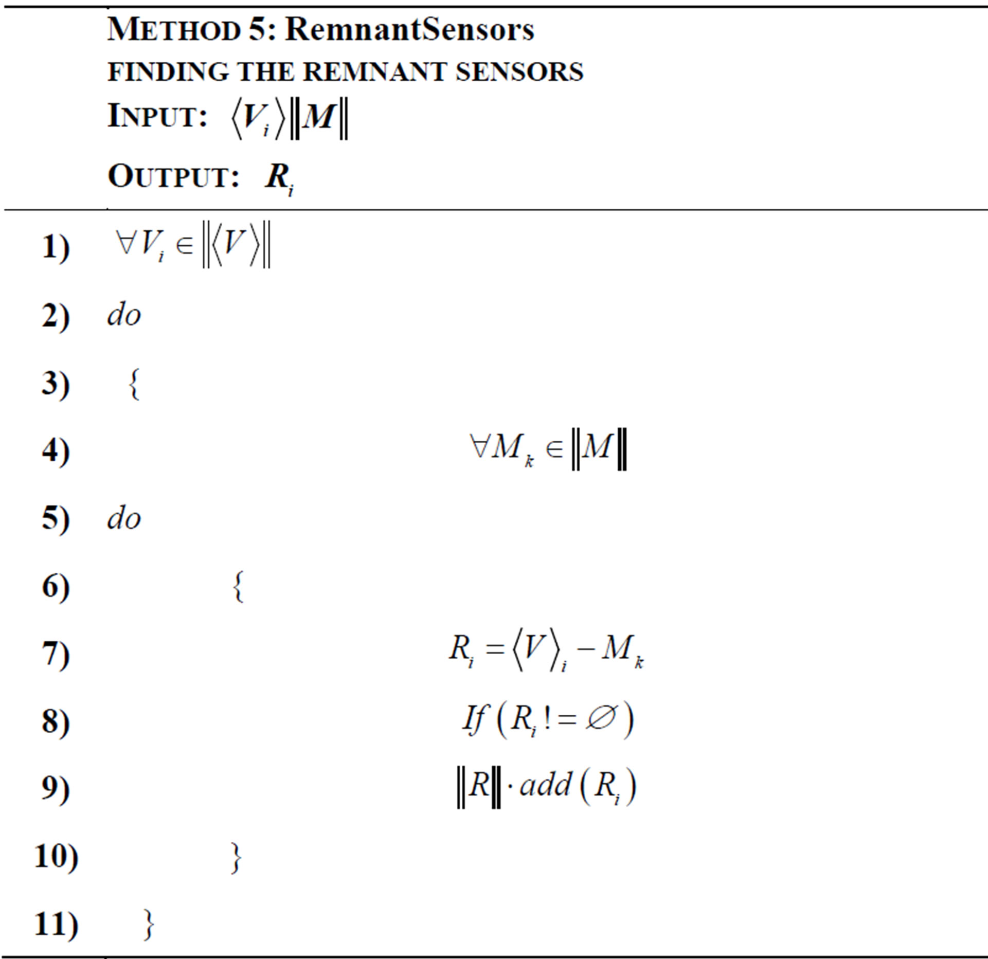
Remnant Sensors
In the Method 5, RemnantSensors, the inputs are , a list of matched groups, and
 , ungrouped vector. The output is a list of remnant sensors
 . The first step is to find the union of matching direct groups associated with the ungrouped vector, and to list them in (unionMembersOfGroup), then find the interaction of (unionMembersOfGroup) with the vector’s sensors.
Solid Vector
Most of the sensors in the solid vector do not exist in the direct groups. This vector runs as a filter for ungrouped vector, and only those sensors which appear in the solid vector can appear in the ungrouped vector as well. See Method 6.
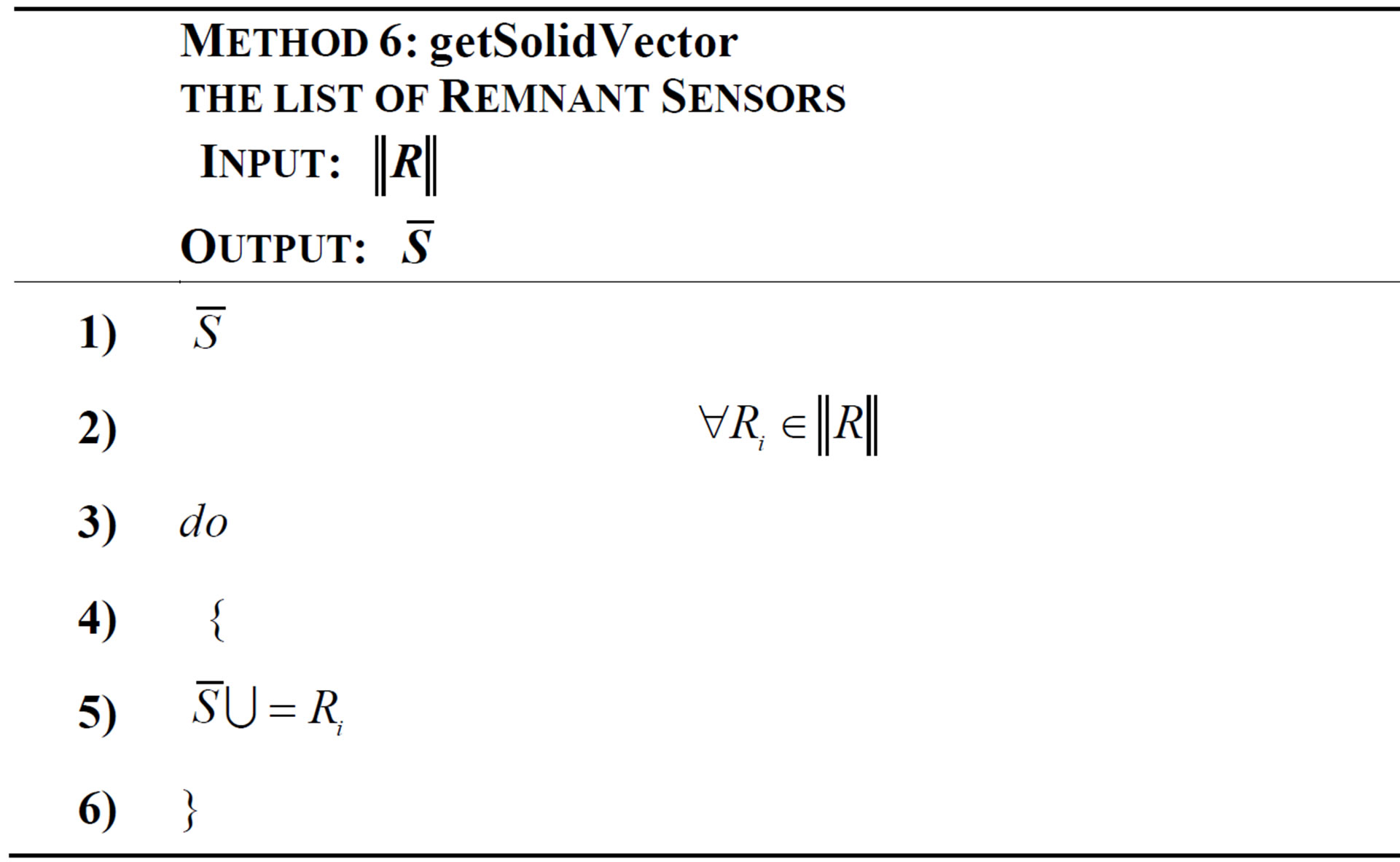
Filtered Vectors
After filtering all ungrouped vectors, we can continue counting the repetition of all filtered ungrouped vectors until we find new direct groups. In Method 7, the inputs are , a solid vectors, and
 , a list of ungrouped vectors. The output is a list of vectors contains only those sensors that appeared in the solid vector.