Wireless Sensor Network
Vol.4 No.9(2012), Article ID:22509,7 pages DOI:10.4236/wsn.2012.49032
Neighbor-Based Malicious Node Detection in Wireless Sensor Networks
Department of Computer Engineering, Hongik University, Seoul, Korea
Email: yhchoi@cs.hongik.ac.kr
Received June 26, 2012; revised July 30, 2012; accepted August 5, 2012
Keywords: Wireless Sensor Networks; Malicious Nodes; Faults; Neighbor-Based Detection
ABSTRACT
The primary function of wireless sensor networks is to gather sensor data from the monitored area. Due to faults or malicious nodes, however, the sensor data collected or reported might be wrong. Hence it is important to detect events in the presence of wrong sensor readings and misleading reports. In this paper, we present a neighbor-based malicious node detection scheme for wireless sensor networks. Malicious nodes are modeled as faulty nodes behaving intelligently to lead to an incorrect decision or energy depletion without being easily detected. Each sensor node makes a decision on the fault status of itself and its neighboring nodes based on the sensor readings. Most erroneous readings due to transient faults are corrected by filtering, while nodes with permanent faults are removed using confidence-level evaluation, to improve malicious node detection rate and event detection accuracy. Each node maintains confidence levels of itself and its neighbors, indicating the track records in reporting past events correctly. Computer simulation shows that most of the malicious nodes reporting against their own readings are correctly detected unless they behave similar to the normal nodes. As a result, high event detection accuracy is also maintained while achieving a low false alarm rate.
1. Introduction
In a wireless sensor network, operating in a harsh and unattended environment, sensor nodes may generate incorrect sensor readings and wrong reports to their neighbors, causing incorrect decisions or energy depletion. The potential sources of incorrect readings and reports include noise, faults, and malicious nodes in the network. Unlike noise and faults, malicious nodes can arbitrarily modify the sensed data and intentionally generate wrong reports. To ensure a reliable event detection in the presence of such wrong data and reports, it is necessary to detect and isolate malicious nodes, greatly reducing their impact on decision-making.
Several fault detection schemes for wireless sensor networks have been proposed in the literature [1-5]. They use centralized, distributed, or hierarchical models. Due to the communication overhead most schemes employ a distributed model, using either neighbor coordination or clustering. As the fault or error models for detection, noise and a few types of faults, such as transient and permanent faults, are typically used. Malicious nodes, however, can generate arbitrary sensor readings which do not conform to the typically used fault models. In that case, the resulting malicious node detection rate becomes much poorer than the estimated one.
Rajasegarar et al. presented an overview of existing outlier detection schemes for wireless sensor networks [6]. Sensor readings that appear to be inconsistent with the remainder of the data set are the main target of the detection. Curiac et al. [7] proposed a detection scheme using autoregression technique. Signal strength is used to detect malicious nodes in [8], where a message transmission is considered suspicious if the strength is incompatible with the originator’s geographical position. Xiao et al. developed a mechanism for rating sensors in terms of correlation by exploring Markov Chain [9]. A network voting algorithm is proposed to determine faulty sensor readings.
Atakli et al. [10] presented a malicious node detection scheme using weighted trust evaluation for a three-layer hierarchical network architecture. Trust values are employed to identify malicious nodes behaving opposite to the sensor readings. They are updated depending on the distribution of neighboring nodes. An improved intrusion detection scheme based on weighted trust evaluation was proposed in [12]. The mistaken ratio of each individual sensor node is used in updating the trust values. Trust management schemes have been proposed in routing and communications [13]. Some efforts are also being made to combine communication and data trusts [14]. However, malicious node detection in the presence of various types of misleading sensor readings due to the compromised nodes have not been deeply investigated. In addition, the resulting event detection performance has not sufficiently been taken into account in malicious node detection.
In this paper, we present a neighbor-based malicious node detection scheme for wireless sensor networks. Malicious nodes are modeled as faulty nodes that may intentionally report false data with some intelligence not to be easily detected. The scheme identifies malicious nodes unless they behave similar to normal nodes. Confidence levels and weighted majority voting are employed to detect and isolate malicious nodes without sacrificing normal nodes and degrading event detection accuracy.
2. Network Model and Operating Modes
In presenting our neighbor-based malicious node detection scheme we use a flat network where sensor nodes are deployed randomly in the sensor field. All the sensor nodes are assumed to have the same transmission range r. Hence two nodes are neighbors of each other if their distance is less than or equal to r. Each sensor node detects malicious nodes along with faulty nodes based on its own sensor readings and those of its neighboring nodes.
In detecting malicious nodes, two different modes of operation are employed: event-driven and periodic, as shown in Figure 1, where Tc denotes the period. In the figure, ts is the interval between two consecutive sensor readings and . In the event-driven mode, sensor nodes with an unusual reading send an alarm to their neighbors. In the periodic mode, on the other hand, each sensor node periodically sends a report to its neighbors, regardless of the occurrence of an event.
The reason for employing the periodic mode is to maintain high quality fault management without a significant increase in power consumption. In event-driven mode, no diagnostic checking is performed until an unusual sensor reading occurs, resulting in delayed or inaccurate fault management unless alarms, due to malicious nodes, faults, and events, are generated sufficiently often. In the added periodic mode, some communication faults and nodes with a stuck-at-0 (normal) fault, to be addressed shortly, are to be detected with a manageably small delay. Since internode communications are involved in periodic mode, the period, Tc, should be long enough
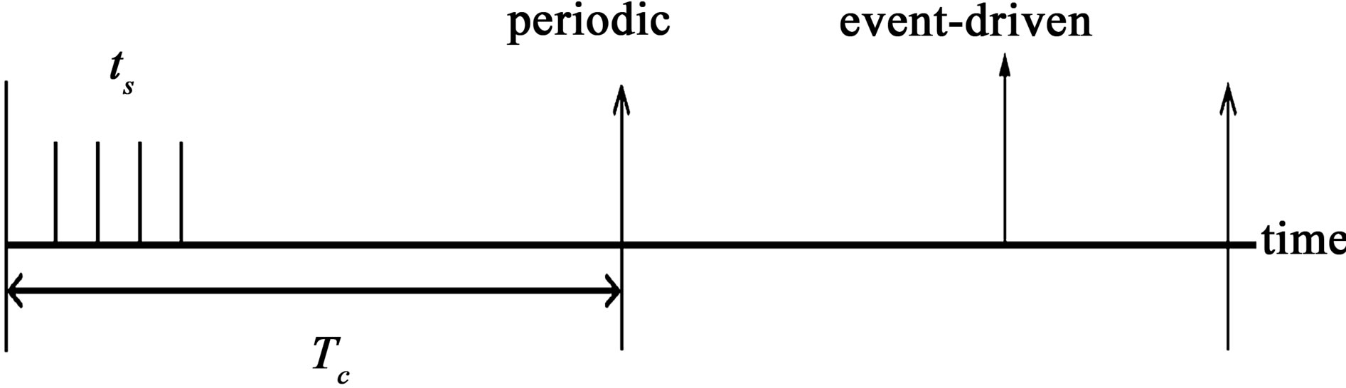
Figure 1. Two different modes of operation.
to reduce the required power consumption. Power consumption can be made negligibly small if a relatively large Tc is good enough to play the diagnostic role, even without degrading malicious node or event detection performance as compared to more frequent checking.
3. Modeling Malicious Nodes
Sensor networks, deployed in an unattended mode, are likely to have malicious nodes, caused by an attack. In general, an attacker can launch a number of attacks against a sensor network as shown in the literature [11]. Most research has investigated direct attacks against the networks and proposed some techniques for detecting or preventing such attacks. In this paper, we focus on indirect attacks where the malicious nodes behave normally but report only false sensor readings to neighbors to mislead the network to reach an incorrect decision, causing serious consequences, or to waste energy due to unnecessary computing and communication.
Sensor readings can also be unusual due to noise, faults, and events. Hence malicious nodes must be detected in the presence of such faults and events. To deal with the malicious nodes, we treat them as faulty nodes that can arbitrarily modify their readings. Simply reporting against their own readings might quickly break down the network function unless some fault-tolerance measures are taken. Such a trivial malicious behavior, however, can be detected even with a simple detection scheme, unless they are clustered.
Prior to modeling malicious nodes, we first define models for faults and events. We assume that faults may occur in any nodes in the network and all sensor nodes are faulty with the same probability. Each sensor node is assumed to know the range of normal readings, and it thus can determine whether the sensor readings belong to the normal range. Here we define “normal” range to be the range of correct sensor readings in the case of noevents. All other readings outside the normal range are named “unusual” for convenience. Hence correct readings at a good sensor node in an event region are also called “unusual”. In addition, each sensor reading is assumed to be binary and it thus is either 0 (normal) or 1 (unusual). Two types of faults, transient and permanent, are considered in this paper. Both transient and permanent faults are assumed to occur, randomly and independently, at all nodes with the same probabilities of pt and pp, respectively. Nodes with transient faults should be treated as normal nodes, even though they sometimes exhibit incorrect readings. Sensor nodes with a permanent fault may report a 0 or 1, repeatedly. Such faults are named stuck-at-0 and stuck-at-1 faults for convenience. They are assumed to occur with the same probability (i.e.
 ).
).
Malicious nodes are also assumed to occur randomly and independently with the same probability pm. They may report any value, either 0 or 1, regardless of the actual sensor reading. In modeling malicious nodes, we assume that they report against their readings with probability pma. If pma = 0.7, for example, malicious nodes report against their readings with a probability of 0.7.
Under the simplifying assumption that pt is symmetric, i.e. P(1|no-event) = P(0|event), the probability that a malicious node reports differently from the ground truth, Pinv, can be written as Pinv = pt(1 – pma) + (1 – pt)pma. For a given pt (<0.5) the value of Pinv increases with pma. If pt = 0.2 and pma = 0.2, for example, Pinv = 0.32, a little higher than pt. If pma increases to 0.8, Pinv = 0.68, significantly higher than pt. If pma is reduced to 0.1, Pinv = 0.26, very close to pt. In that case, it is not easy to distinguish malicious nodes from normal nodes. Although malicious nodes behaving like a normal node might remain undetected, they do not significantly affect the system performance.
Our scheme is focused on detecting malicious node behaving differently from normal nodes, while maintaining high event detection performance even in the face of malicious nodes. Event detection in the presence of malicious nodes becomes more complicated since added incorrect readings due to malicious nodes might lead to poor event detection accuracy and increased false alarms.
4. Neighbor-Based Malicious Node Detection
In detecting malicious nodes in the presence of faults and events, we employ a smoothing filter and confidence level evaluation to enhance the malicious node detection rate. A filter is used to correct some false readings due to transient faults. It thus effectively reduces the transient fault probability pt in such a way that malicious nodes can be detected for a wider range of pma. Confidence levels are employed to estimate the trustworthiness of sensor nodes, reflect the levels in decision making process, and logically isolate malicious nodes and nodes with a permanent fault from the network.
4.1. Data Smoothing and Variation Test
In the periodic and event-driven detection, the readings, affected by transient faults, might cause an incorrect decision, resulting in the waste of resources, in both computation and communication. In addition, the diagnostic results influenced by transient faults might lead to the isolation of some normal sensor nodes from the network and loss of sensing coverage.
In order to avoid unnecessary event-driven detection cycles and incorrect decisions due to transient faults, we employ a filter, as shown in Figure 2, to smooth out the sensor readings in such a way that most transient overshoots can be removed not to cause unwanted alarms. In the figure, the sensor reading  of node vi at time t = k is given to the range test block to produce a binary value
  (i.e. 0 or 1) and then applied to the smoothing filter to generate the output
 . The range test block checks to see if the input belongs to the normal range. The same input
  is also given to the variation test block to see if the variation of (filtered if necessary) sensor readings,
 , during the period of Tc,
 , is less than δ for all the values of k in the cycle. A flag Si at the sensor node vi is set to 1 if the condition is met. The variation test can be applied to applications where the readings of a normal sensor, in the case of no-event, vary in such a way that the variation during the given period Tc is greater than or equal to δ. The readings of a temperature sensor, where Tc is a day, for example, may change such that the variation is likely to be greater than or equal to δ (say δ = 3). This variation test might detect some nodes with stuckat-0 (normal) faults which affect negatively when they are in an event region.
The filter performs the following smoothing function using w most recent readings with a threshold q as follows:
 = 1 for
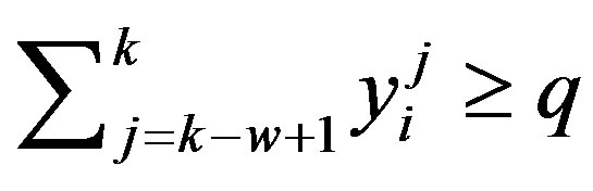
Some other filters may be used without modification of the rest of the scheme. The smoothing function is performed within the sensor node, requiring no internode communications. Internode communications are needed once every test cycle of Tc (i.e. periodic) or when  =1 (i.e. event-driven). In the event-driven mode, only the nodes receiving an alarm from their neighbors locally perform an event detection process to make a decision on the correctness of the alarm.
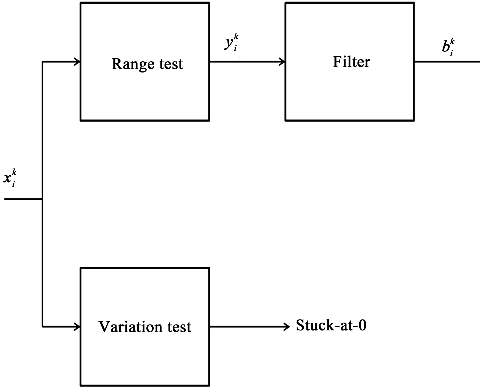
Figure 2. Data smoothing and variation test.
The reduction of incorrect readings due to transient faults improves the malicious node detection performance. Permanent faults, unless the number of such faults is negligibly small, also needs to be removed from the network, to enhance the network reliability. Since the number of faulty nodes increases with time, it is desirable to isolate them upon detection. Confidence levels to be addressed in the next subsection help detect nodes with a permanent fault and malicious nodes.
4.2. Confidence Level Evaluation
To cope with the malicious node problem, we model a sensor network as a weighted digraph, where each sensor node vi has wij , ranging from 0 to 1, initialized to 1, as the confidence level of its neighboring node vj from the viewpoint of vi. The level wij is updated at node vi based on vj’s report and the decision made at vi on an event. If wij = 1, for example, node vi totally trusts node vj. If wij = 0, however, vi does not trust vj at all. Similarly, each node vi has its own confidence level, wii, also ranging from 0 to 1. Once wii reaches 0, the fault status of vi, Fi, is set to 1, indicating that vi is faulty.
The confidence levels defined above represent the trustworthiness of the corresponding sensor readings and are reflected in the proposed neighbor-based malicious node detection scheme to be addressed shortly. At the end of each event-driven and periodic detection cycles, each sensor node updates its own confidence level and those of its neighbors to reflect the levels in the subsequent decision making process. Moreover, they are used to identify malicious nodes.
Updating the confidence levels has the following purposes. Each sensor node with a permanent fault quickly loses its confidence levels from its normal neighbors, and it will then be isolated from the rest of the network. In addition, a malicious node reporting against its own readings in such a way that its behavior is away from normal nodes' behavior also loses its confidence levels from its neighbors to be eventually detected. The policies of updating confidence levels are described in detail in the next subsection.
4.3. Malicious Node Detection
In our neighbor-based detection scheme, each sensor node detects malicious nodes, along with faulty nodes, locally using only the sensor readings of its neighboring nodes. A weighted majority voting using the confidence levels as weights is used to detect malicious nodes. The proposed detection scheme can be depicted as follows.
Malicious Node Detection 1) Given sensor reading , obtain
  and determine
 , and perform variation test for suck-at-0 fault detection 2) Receive
  and Fj from neighbors (periodic). Send an alarm to neighboring nodes (event-driven)
3) Compute and make a decision Di
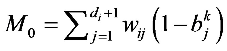 and
and 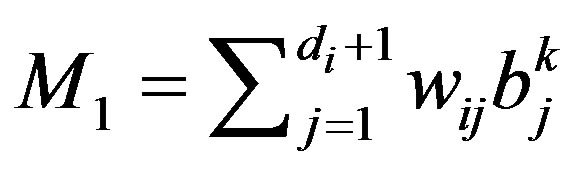
Di = 1 (i.e. an event) if M1 > M0
4) Update the confidence levels wij accordingly In Step 1, most wrong data due to transient faults are locally corrected and hence false alarms can be greatly reduced without incurring any internode communications. In addition, the variation test is conducted for the sensor readings during the cycle Tc. In Step 2, neighbor communications are used to perform periodic checking (in the periodic mode). In the event-driven mode, however, only the nodes with bi = 1 report an alarm to neighboring nodes to initiate an event-driven detection. Step 3 performs a weighted majority voting to make a decision on an event, where M1 (M0) is the sum of weights of nodes with bij = 1(0) and di is the node degree of vi. The confidence levels are reflected in the decision making process. In Step 4, all the weights, wij , are updated. Updating the weights in such a way that malicious nodes can be effectively removed from the network is important.
Our updating policy differs depending on the decision made on an event. In the case of no-event, the weight wij is updated as shown in Table 1, where Fj denotes the fault status of vj. The confidence level of node vj, wij, is increased by β only when vj is fault-free (i.e. Fj = 0) and it belongs to the majority group. It is decreased by α otherwise. Here α and β have to be properly chosen to optimize the performance.
In the case of an event, the weight wij is updated as shown in Table 2. The only difference is the third row where the confidence level remains unchanged since the exact boundary of an event region is unknown.

Table 1. Updating wij at node vi in case of no-event.

Table 2. Updating wij at node vi with Di = 1 in case of an event.
Each sensor node vi also updates its own confidence level wii in the case of no-event as follows.
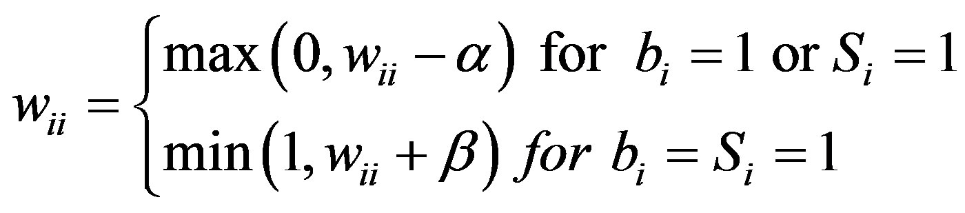
In the above expression, Si = 1 means that the readings at node vi do not satisfy the minimum variation requirements, indicating a potential stuck-at-0 fault. Fault status of node vi, Fi, initially 0 (fault-free), is set to 1(faulty) when wii reaches 0. Once it is set to 1, it will stay there if no recovery action is taken.
Malicious nodes behaving like a normal node can hardly be detected. However, it does not cause a significant problem. Malicious nodes with some intelligence might behave differently from normal and faulty nodes to remain undetected. The proposed scheme is focused on accurately detecting such malicious nodes and isolating them from the network. Consequently, it achieves high performance for a wider range of pma.
5. Simulation Results
Computer simulation is conducted to evaluate the effectiveness of our malicious node detection scheme and the resulting event detection accuracy. In the simulation, we randomly deployed 1024 sensor nodes in a square area. The transmission range r is chosen to set the average node degree d to be 12. In addition, an event region is assumed to be a circle with radius r (i.e. the same as the transmission range).
Transient faults, permanent faults, and malicious nodes are generated randomly and independently. In the case of permanent faults, they are generated uniformly during the first 10 cycles of operation. In the case of no event, malicious nodes are assumed to report against the actual readings with probability pma. On the other hand, they are assumed to report a 0 when they are in an event region, to estimate the event detection performance in the worst case.
Two metrics, malicious node detection rate (MDR) and misdetection rate (MR), are defined to evaluate the proposed malicious node detection scheme. MDR is defined to be the ratio between the number of detected malicious nodes and the total number of malicious nodes. MR is defined as the ratio of normal nodes determined to be faulty to the total number of normal nodes. The reason for not defining MR with respect to malicious nodes is that malicious nodes behaving like a normal node (i.e. reporting correctly most of the time) do not harm at all until they change their behavior.
Two additional metrics, event detection accuracy (EDA) and false alarm rate (FAR), are used to evaluate the resulting event detection performance. EDA is defined as the ratio between the number of events correctly identified and the total number of events generated. FAR is the ratio of the number of nodes reporting a 1 to the total number of nodes, in case of no-event We first performed simulation to estimate MDR and MR for four different values of pm, 0.05, 0.10, 0.15, and 0.20, when pp = 0.1, pt = 0.1, pma = 0.4. The results, after 50 cycles of operation, are shown in Table 3(a), where α = 0.2 and β = 0.05 are chosen. For comparison purposes, we also performed simulation for α = β = 0.1 (Table 3(b)). MDR in Table 3(a) is high while MR is negligibly small. On the other hand, MDR in Table 3(b) is extremely low due to the fact that confidence levels lost are quickly recovered. As can be seen in Table 3, the value of  has to be assigned properly to achieve high MDR, while maintaining low MR. If
  = 4, for example, a malicious node sending an alarm every five cycles in case of no-event recovers its confidence levels, and is thus unlikely to be detected. Such a high MDR in Table 3(a) is obtained since pma is set to 0.4 in the simulation.
The confidence level of a malicious node becomes lowered with time to reach the lower bound if
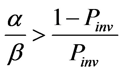 . If pma = 0.2, for example, Pinv = 0.26, resulting in
 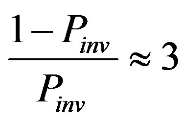 That is, the node is expected to report a 1 every four cycles on average in the case of noevent. Even in that case,
  = 4 is sufficient to lower the confidence levels of malicious nodes to be eventually detected.
In Figure 3, the resulting EDA is shown for various values of pm for the same values of α and β. FAR for the two different cases are almost the same and very close to 0, and are not shown in the figure. The first pair (0.2, 0.05) maintains more persistent and stable performance compared to the other pair (0.1,0.1) as pm increases.
In order to see the importance of the values of α and β in malicious node detection, we conducted the same
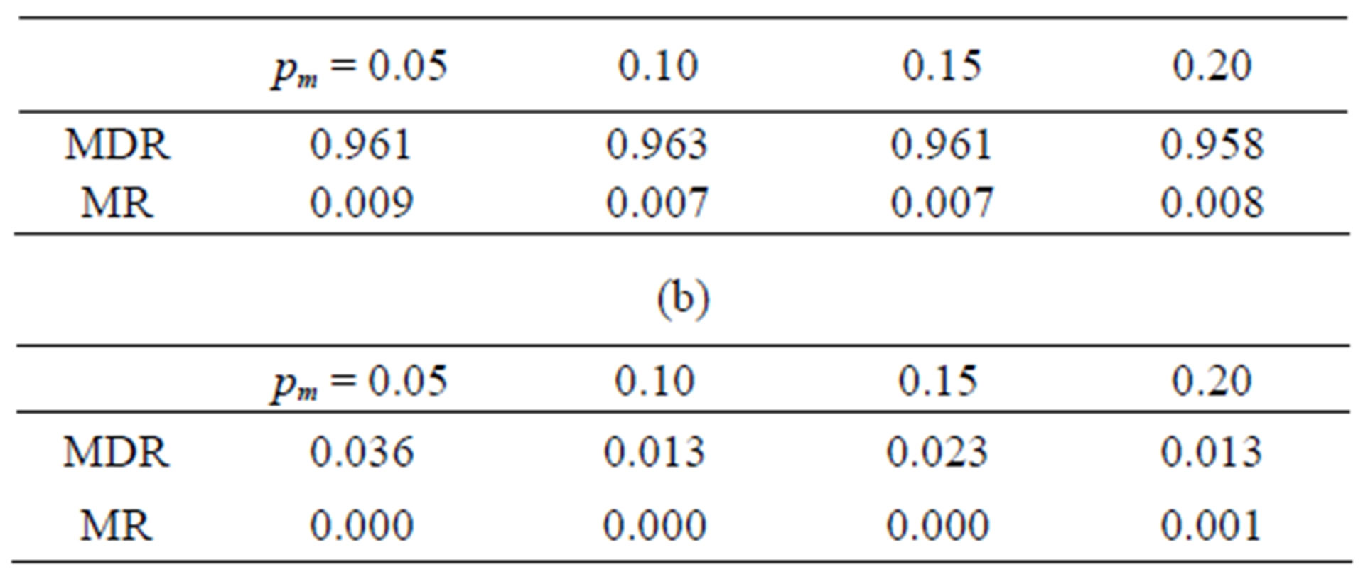
Table 3. MDR and MR for various values of pm when pp = pt = 0.1. (a) α = 0.2, β = 0.05; (b) α = 0.1, β = 0.1.
simulation for five different values of pma. Two pairs of (α, β), (0.2,0.02) and (0.2,0.05) are chosen for comparison purposes. For pp = 0.1, pt = 0.1, and pm = 0.2, the resulting MDR and EDA are shown in Figure 4. MR and FAR are not included since they are close to 0 for the cases under consideration.
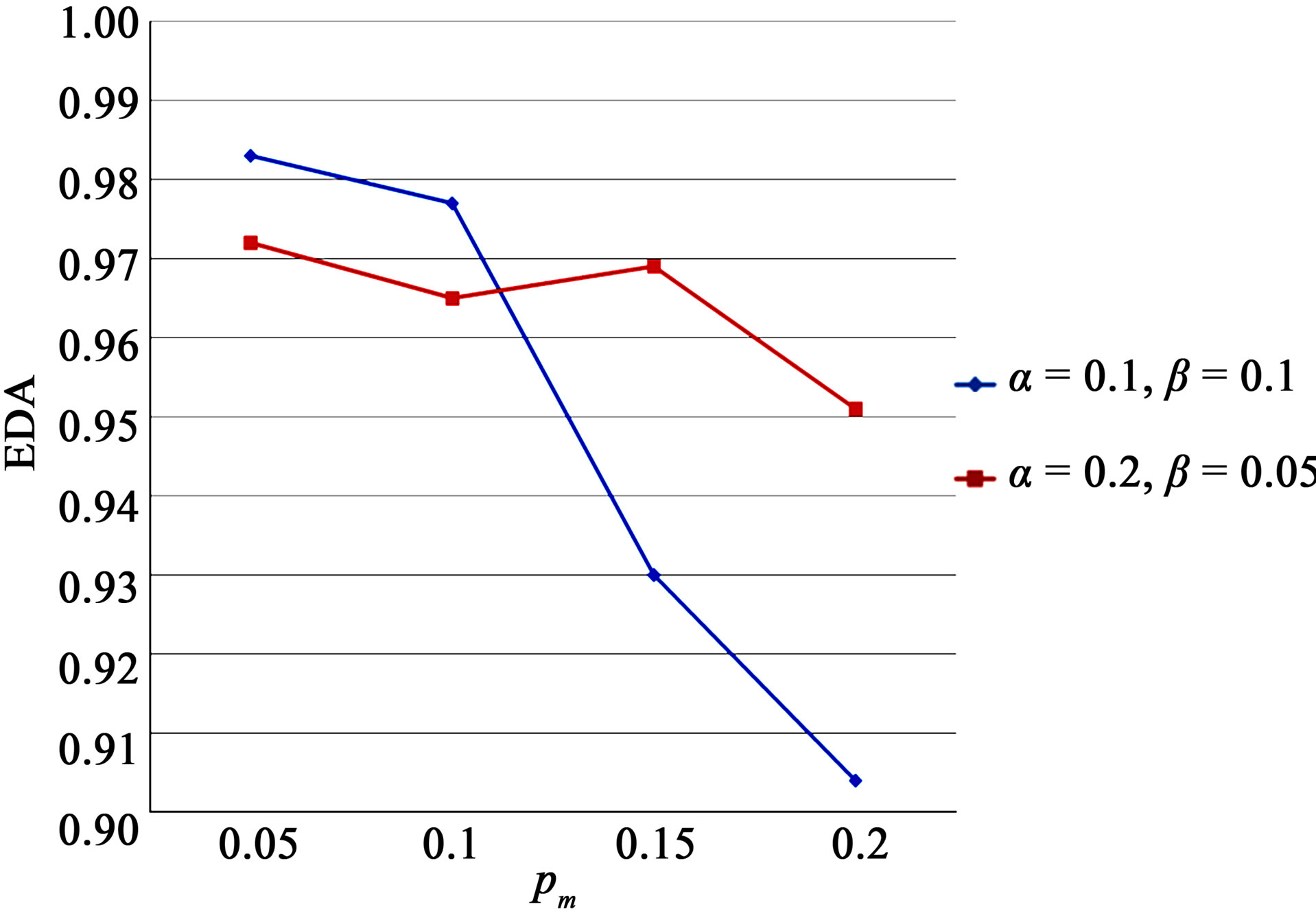
Figure 3. EDA for two different pairs of α and β.
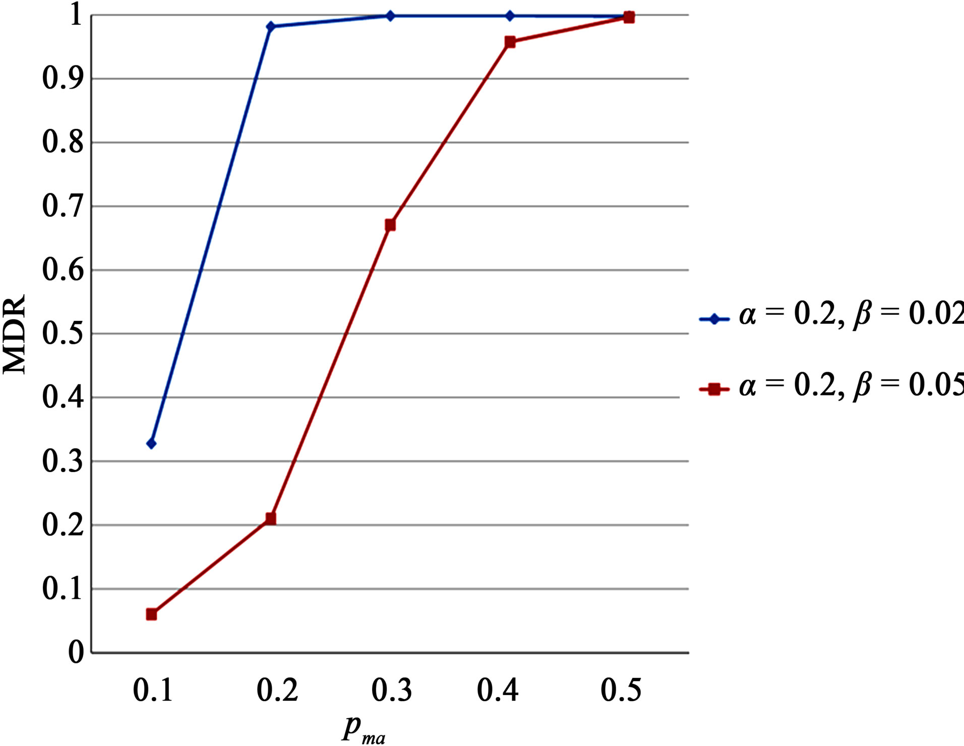
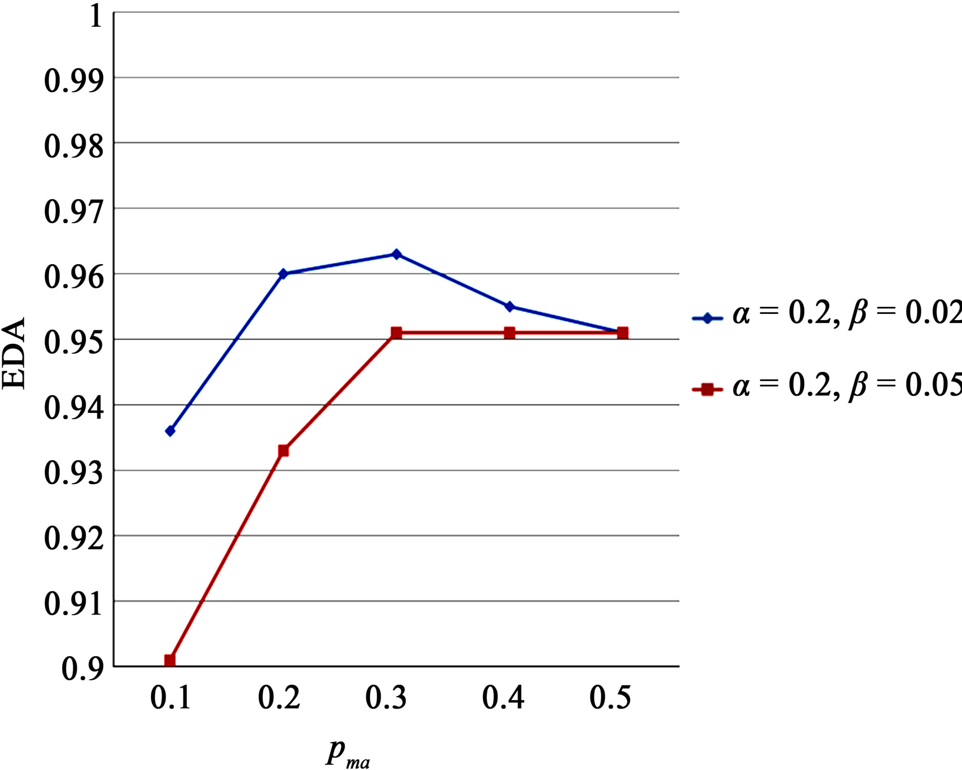
Figure 4. EDA for two different pairs of α and β.
As can be seen from Figure 4, MDR for (0.2,0.02) is significantly higher than that for (0.2,0.05) for relatively small values of pma. These improvements have been made by increasing  without sacrificing normal nodes. For pt = 0.1, if pma is close to 0.1, malicious nodes behave like a normal node, and thus they can hardly be detected without increasing the detection time or sacrificing some normal nodes. Filtering transient faults lowers pt in such a way that a considerable amount of malicious nodes can still be detected.
We then conducted simulation to see the performance gain we can obtain by removing stuck-at-0 nodes. The proposed scheme has provisions to detect such faults as long as the resulting sensor readings are confined to a relatively small range of normal values over time compared to normal sensor nodes. Since not all stuck-at-0 faults meet the requirements, the scheme is partially effective. The simulation results for various values of pp when stuck-at-0 faults are isolated are shown in Table 4(b), where α = 0.2, β = 0.05 and pma = 0.4 are chosen. For comparison purposes the results when stuck-at-0 faults remain in the network are shown in Table 4(a).
As far as MDR and MR are concerned, there are negligible differences in performance. A notable difference in EDA, however, is observed as pp increases. Removing stuck-at-0 faults is desirable when EDA is concerned.
Finally, we evaluated the proposed scheme in terms of EDA and FAR by comparing its performance with those of majority voting (MV). Since MV is not for malicious node detection, MDR and MR are not included in the comparisons. The results for two different values of pp when pm = pt = 0.1 are shown in Table 5, where α = 0.2, β = 0.05, and pma = 0.4 are chosen for our scheme. The proposed scheme outperforms the majority voting with respect to EDA and FAR.

Table 4. MDR, MR, EDA, and FAR for various values of pp when pm = pt = 0.1. (a) Without removing stuck-at-0 faults; (b) after removing stuck-at-0 faults.
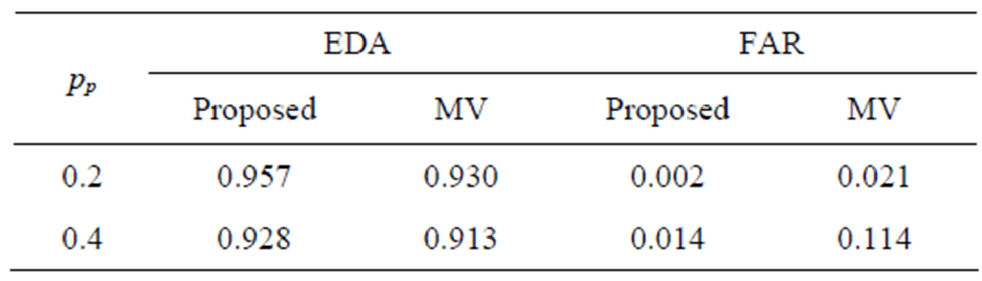
Table 5. EDA and FAR for two different values of pp when pm = pt = 0.1.
6. Conclusion
In this paper, we proposed a neighbor-based malicious node detection scheme for wireless sensor networks. Malicious nodes are detected in the presence of faults and events without sacrificing normal nodes. They are modeled as faulty nodes that can arbitrarily modify sensor readings and behave intelligently not to be easily detected. Confidence levels are used to estimate trustworthiness of sensor nodes during normal operation. They are reflected in the decision making process at each sensor node. Two parameters for updating the confidence levels are employed to distinguish malicious nodes from normal modes as long as they behave differently from normal nodes. The ratio between them needs to be properly chosen to eventually isolate malicious nodes even if they behave slightly differently from normal nodes. Both detection and misdetection rates are maintained high and low, respectively, in the face of faults and events. The resulting event detection accuracy is kept high while maintaining low false alarm rates.
7. Acknowledgements
This research was supported by the National Research Foundation of Korea (NRF) Grant funded by the Korean Government (NRF-2011-0007187).
REFERENCES
- M. Yu, H. Mokhtar and M. Merabti, “Fault Management in Wireless Sensor Networks,” IEEE Wireless Communications, Vol. 14, No. 6, 2007, pp. 13-19. doi:10.1109/MWC.2007.4407222
- H. S. Hu and G. H. Qin, “Fault Management Frameworks in Wireless Sensor Networks,” 4th International Conference Intelligent Computation Technology and Automation, Shenzhen, 28-29 March 2011, pp. 1093-1096. doi:10.1109/ICICTA.2011.559
- C.-R. Li and C.-K. Liang, “A Fault-Folerant Event Boundary Detection Algorithm in Sensor Networks,” Information Networking: Towards Ubiquitous Networking and Services, Vol. 5200, 2008, pp. 406-414. doi:10.1007/978-3-540-89524-4_41
- X. H. Xu, B. Zhou and J. Wan, “Tree Topology Based Fault Diagnosis in Wireless Sensor Networks,” International Conference on Wireless Networks and Information Systems, Shanghai, 28-29 December 2009, pp. 65-69.
- M. H. Lee and Y.-H. Choi, “Fault Detection of Wireless Sensor Networks,” Computer Communications, Vol. 31, No. 14, 2008, pp. 3469-3475. doi:10.1016/j.comcom.2008.06.014
- S. Rajasegarar, C. Leckie and M. Palaniswami, “Anomaly Detection in Wireless Sensor Networks,” IEEE Wireless Communications, Vol. 15, No. 4, 2008, pp. 34-40. doi:10.1109/MWC.2008.4599219
- D. I. Curiac, O. Banias, F. Dragan, C. Volosencu and O. Dranga, “Malicious Node Detection in Wireless Sensor Networks Using an Autoregression Technique,” 3rd International Conference on Networking and Services, Athens, 19-25 June 2007, p. 83.
- W. Junior, T. Figueiredo, H. Wong and A. Loureiro, “Malicious Node Detection in Wireless Sensor Networks,” 18th International Parallel and Distributed Processing Symposium, 26-30 April 2004, New Mexico, p. 24.
- X.-Y. Xiao, W.-C. Peng, C.-C. Hung and W.-C. Lee, “Using Sensor Ranks for In-Network Detection of Faulty Readings in Wireless Sensor Networks,” International Workshop Data Engineering for Wireless and Mobile Access, Beijing, 10 June 2007, pp. 1-8. doi:10.1145/1254850.1254852
- I. M. Atakli, H. Hu, Y. Chen, W.-S. Ku and Z. Su, “Malicious Node Detection in Wireless Sensor Networks Using Weighted Trust Evaluation,” Proceedings of Spring Simulation Multi-Conference, Ottawa, 14-17 April 2008, pp. 836-843.
- X. Chen, K. Makki, K. Yen, and N. Pissinou, “Sensor Network Security: A Survey,” IEEE Communication Surveys & Tutorials, Vol. 11, No. 2, 2009, pp. 52-73. doi:10.1109/SURV.2009.090205
- L. Ju, H. Li, Y. Liu, W. Xue, K. Li and Z. Chi, “An Improved Detection Scheme Based on Weighted Trust Evaluation for Wireless Sensor Networks,” Proceedings of the 5th International Conference on Ubiquitous Information Technology and Applications, Sanya, 16-18 December 2010, pp. 1-6.
- M. Momani and S. Challa, “Survey of Trust Models in Different Network Domain,” International Journal Ad Hoc, Sensor & Ubiquitous Computing, Vol. 1, No. 3, 2010, pp. 1-19.
- M. Momani, S. Challa and R. Alhmouz, “Can We Trust Trusted Nodes in Wireless Sensor Networks?” International Conference Computer and Communication Engineering, Kuala Lumpur, 13-15 May 2008, pp. 1227-1232.