Journal of Water Resource and Protection
Vol.4 No.7(2012), Article ID:19770,9 pages DOI:10.4236/jwarp.2012.47049
SWAT Model Application to Assess the Impact of Intensive Corn-Farming on Runoff, Sediments and Phosphorous Loss from an Agricultural Watershed in Wisconsin
USEPA Office of Research and Development’s Landscape Ecology Branch, Las Vegas, USA
Email: yuan.yongping@epa.gov
Received February 13, 2012; Revised March 28, 2012; accepted April 29, 2012
Keywords: Watershed Modeling; SWAT; Runoff; Sediment Yield; Phosphorus Loss; BMPs
ABSTRACT
The potential future increase in corn-based biofuel may be expected to have a negative impact on water quality in streams and lakes of the Midwestern US due to increased agricultural chemicals usage. This study used the SWAT model to assess the impact of continuous-corn farming on sediment and phosphorus loading in Upper Rock River watershed in Wisconsin. It was assumed that farmers in the area where corn was rotated with soybean would progressively skip soybean for continuous corn as corn became more profitable. Simulations using SWAT indicated that conversion of corn-soybean to corn-corn-soybean would cause 11% and 2% increase in sediment yield and TP loss, respectively. The conversion of corn-soybean to continuous corn caused 55% and 35% increase in sediment yield and TP loss, respectively. However, this increase could be mitigated by applying various BMPs and/or conservation practices such as conservation tillage, fertilizer management and vegetative buffer strips. The conversion to continuous corn tilled with conservation tillage reduced sediment yield by 2% and did not change TP loss. Increase in P fertilizer amount was roughly proportional to increase in TP loss and 11% more TP was lost when fertilizer was applied four months before planting. Vegetative buffer strips, 15 to 30 m wide, around corn farms reduced sediment yield by 51% to 70% and TP loss by 41% to 63%.
1. Introduction
Nutrient runoff from US farm lands has been linked to deterioration of water quality in water bodies downstream, especially lake eutrophication and estuarine hypoxic zones [1]. As of 2004, the USEPA reported that 44% of assessed stream length, 64% of assessed lake area, and 30% of estuarine area were impaired to a level unsuitable to support fish and unsuitable for swimming [2]. High oil prices, the desire to reduce the US dependency on foreign oil and potential increase in US agricultural profitability have triggered a need to generate biofuels from annual crops, especially corn. From 2002 to 2006 alone US ethanol production increased 125% [3]. This corn intensive farming could potentially exacerbate water, air and soil pollution since corn requires higher amounts of agricultural chemicals (nitrogen and phosphorus fertilizers, and pesticides) and tillage than some other crops [4]. In the Midwestern US many lakes suffer from excessive growth of harmful algae, believed to be promoted by excessive loss of phosphorus (P) from agricultural farms [5]. Control and reduction of P could reduce eutrophication in lakes since P is a growth-limiting nutrient for harmful algal blooms [6,7]. The amount of P loss from farms to streams is believed to depend mainly on P content of surface soil, type of soil, tillage and crop management [8]. To reduce pollution of water bodies, regulatory agencies such as USEPA and USDA-NRCS promote agricultural best management practices (BMPs) to reduce non-point source pollution: soil erosion, nutrient and pesticide runoff [9]. Studies for various structural (e.g., buffers) and non-structural (e.g., fertilizer management) management practices to control loss of sediment and nutrients have shown mixed results. Some ma nagement practices have proven effective at controlling one pollutant while promoting the loss of another. For instance, Heatwaite et al. (2000) indicated that management of manure to control nitrogen (N) has increased soil P and generated higher P in runoff [10]. Also, they noticed that the no-till method recommended to reduce erosion and P loss could cause increased nitrate leaching.
Vegetative buffers, wetlands and management of fertilizer and manure have been suggested by prior studies to be more effective in reducing sediment and P loss into streams [11,12]. In addition, crop rotation (for instance corn-soybean instead of continuous corn) is known to reduce sediment, nutrient and pesticide loss [13]. Soybean has the ability to fix N and requires low amounts of P fertilizer. Soybean improves soil texture, making it an excellent candidate for no-till, and has low weed and insect nuisance which reduces herbicide and insecticide use. Also, soybean fields dry faster, which in wet areas helps prepare land for corn planting [14]. Agricultural tillage methods also affect water quality differently; switching from conventional tillage to conservation tillage (e.g. 30% residue) or to no-till reduces soil erosion, labor and carbon footprint [15]. Residue left by conser vation tillage improves soil resistance to erosion, especially during non-crop growth periods when canopy that reduces raindrop impact is absent. However, in some places, no-till can increase weeds and insects, reducing crop yield [14]. Soil temperature reduction associated with no-till corn can result in slowing early season growth and lower yields. Leaving residue on poorly drained soils, especially in the wet upper Midwest, can prevent fields from drying out fast enough for April or early May planting of corn [16]. To study the effect of non-point source pollution, water quality and quantity from various US streams is monitored by agencies such as the USGS. However, due to the cost involved in longterm monitoring, there are only a limited number of streams with data. Non-point source watershed models are useful to estimate water quality for non-monitored areas and periods, and to evaluate alternative crop management scenarios [11]. Future scenarios could be important tools for policy makers. The objectives of this study were to: 1) estimate variations in water yield, sediment, and TP loads due to land use changes from cornsoybean to continuous corn as well as from lowly disturbed lands (alfalfa) to continuous corn; 2) assess the impact of tillage operation on water yield, sediment and TP loads; and 3) assess the effectiveness of various BMPs and/or conservation practices to mitigate the adverse impact from intensive corn production. Fertilizer management, conservation tillage, and vegetative buffers were the assessed BMPs. The study area was selected in Upper Rock River Watershed, a watershed with numerous lakes, reservoirs and wetlands in Wisconsin (Upper Rock River watershed). Lakes and reservoirs in this region are prone to eutrophication due to upstream agricultural activities and there is lack of studies on effect of continuous corn and mitigation BMPs for this region. Soil and Water Assessment Tool (SWAT) enabled us to quantify present sediment and phosphorous loads into water bodies, and potential future variations due to land use changes and BMPs application.
2. Methods and Procedures
2.1. SWAT Model Description
SWAT is a physically based watershed-scale model developed by the US Department of Agriculture—Agriculture Research Service (USDA-ARS). It operates on a daily time step and was developed to predict the impact of land management on water, sediment, and agricultural chemicals transport in large, complex watersheds with varying slope, soils, and land use over long periods of time [17,18]. Hydrologic processes simulated by SWAT include evapotranspiration, infiltration, channel transmission losses, channel routing, surface flow, lateral flow, and shallow aquifer and deep aquifer discharge [18,19]. SWAT has a stream routing component and can simulate the fate and transformation of nutrients and pesticides within streams, ponds and reservoirs. Crop biomass, crop residue and its contribution nutrient cycling in an agroecosystem is also clearly depicted in SWAT [18]. The model is capable of generating watershed response at various temporal (daily, monthly, and annual) and spatial (Hydrologic Response Unit or HRU, basin and sub-basin, stream reach) scales [20].
2.2. Description of Watershed
The study watershed is located in the glaciated portion of south central Wisconsin and covers approximately 1291 km2. It includes parts of three counties: Fond du Lac, Dodge and Washington (Figure 1). Its land use consists of 66% agricultural land (corn, soybean, wheat, sorghum, and other), 13% wetlands, 12% forests and grassland, 6% urban land and 3% water. It lies in the Eastern Ridges and Lowlands region with elevations between 213 and 275 meters above sea level. The climate involves cold and snowy winters (low temperatures around –20 degrees Fahrenheit) and warm and humid summers (average temperature around 55 degrees Fahrenheit and highs between 80 and 85 degrees Fahrenheit). Mean annual precipitation is around 760 mm and snow fall around 1016 mm. The predominant soil types include: Lomira, Kidder, Houghton, Varna, Hochheim, and Fox. Special features in the watershed include Horicon marsh and Sinnissippi Lake which covers an area approximately 134 km2 and 12 km2, respectively. The watershed outlet is located at the Hustisford Dam, Hustisford, WI on the Rock River. The USGS monitoring site (USGS 05424082) is also located at the same location. The Hustisford Dam is controlled to keep Sinissippi lake water depth roughly uniform for leisure purposes.
2.3. Description of Model Inputs
The most important SWAT model inputs include the digital elevation model (DEM), land use and land cover,
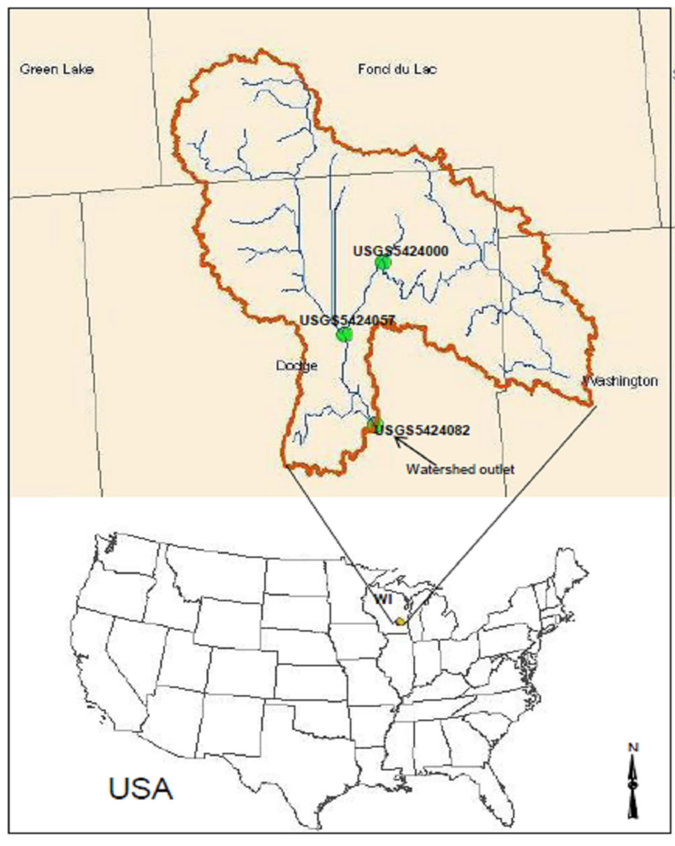
Figure 1. Location of the study watershed.
soil information and weather data. A 30 m by 30 m resolution DEM was used by SWAT to generate the stream network and the watershed boundary. To gain spatiallyexplicit agricultural data which includes information on crop type and rotation, the USGS 2001 National Land Cover Database (NLCD) was expanded by using the USDA National Agriculture Statistical Survey (NASS) Cropland Data Layer (CDL). CDL data collected for years of 2004-2007 were used to expand the “single cultivated crops” land-use within the NLCD into multiple cropping types and rotational information [21]. For soil information, the State Soil Geographic (STATSGO) database embedded in ArcSWAT was used. Daily weather data (1980-2008) from 10 weather monitoring stations inside or in the proximity of the watershed were obtained from NOAA-National Climatic Data Center (NCDC). Hustisford Dam and Horicon Dam operation information was obtained from Village of Hustisford website (www.hustisford.com).
2.4. Model Calibration and Validation
SWAT model performance evaluation consists of comparing model predicted output with measured data. Three quantitative statistics—coefficient of determination (R2), and Nash-Sutcliffe (NSE) and relative error were used for comparison. These methods were recommended by various studies to evaluate the performance of watershed models [22,23]. R2 is a standard regression parameter which shows the strength of the correlation between measured and simulated data. It ranges between 0 and 1, and R2 value equal to 0 indicates no correlation between predicted and measured data while a value equal to 1 indicates that the predicted data perfectly match measured data. NSE is a dimensionless coefficient which shows a relative assessment of the model. The NSE ranges from −∞ to 1 and measures how well the simulated versus observed data match the 1:1 line (Regression line with slope equal to 1). An NSE value of 1 again reflects a perfect fit between the simulated and measured data. A value of 0 or less than 0 indicates that the mean of the observed data is a better predictor than the model output [24]. Normally, satisfactory evaluation criteria are set up depending upon the precision required; R2 and NSE roughly equal to 0.5 were usually recommend by previous studies [22]. When the criteria are not satisfied the next step is to calibrate the model and recheck the performance criteria. Calibration of the model involves the following steps. First, sensitivity analysis is performed to identify key parameters and parameter precision required for calibration. The sensitivity analysis is performed by perturbing input parameters one at a time and comparing their impact on model output; a parameter that causes larger change is deemed more sensitive [25]. Then, model input parameters identified in sensitivity analysis are adjusted so that the model outlet closely resembles monitored data. Data from three USGS sites (05424082, 05428057 and 05424000) were used for calibration and validation. Five years of USGS 0540820 monthly observed data (January 1980 to August 1985) were used for calibration of flow and monthly data from 1998 to 2000 were used for calibration of TP and sediment. Observed monthly data for flow, sediment and TP (1997-2001) from USGS sites 05428057 and 05424000 were used for validation. The reservoir dam operations data were used for reservoir outlet information.
2.5. Description of Simulation Scenarios
SWAT simulation scenarios that were performed in this study (also summarized in Table 1) are as follows:
Corn-soybean land use change scenarios: For the first scenario simulated (base year 2001), the corn-soybean land use (21% of watershed area) was assumed to start with corn at the first year and rotate with soybean the second year. This assumption might not represent the actual distribution of corn and soybean crops but it considers that each crop is rotated once in two-year period for this scenario. As a second scenario, the corn-soybean land use was converted to a rotation of two years corn and third year soybean. A third scenario involved converting corn-soybean land use to continuous corn. The
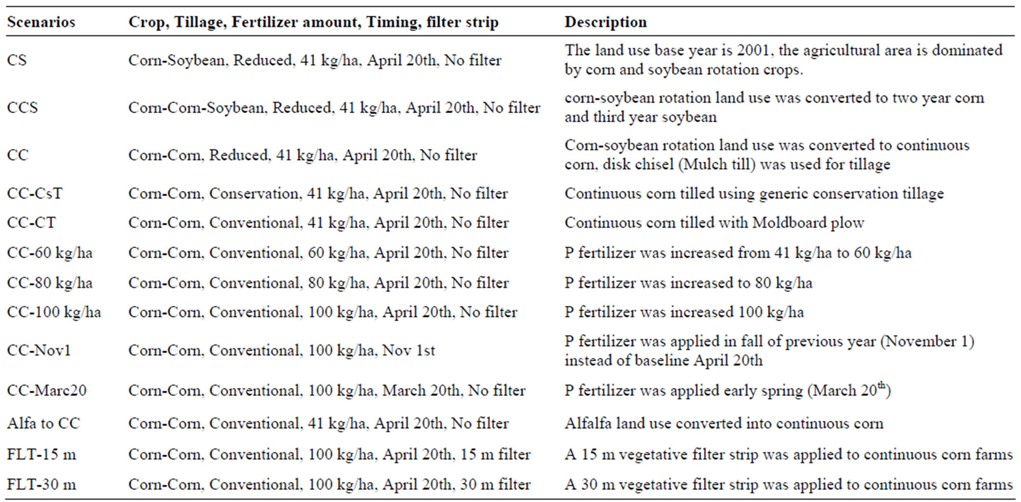
Table 1. Description of simulation scenarios.
fourth scenario involved converting alfalfa land use (7.5% of watershed area) to continuous corn. For the above scenarios corn was planted on May 1st and harvest occurred on October 20th. Fertilizers (at elemental rates of 41 kg P/ha and 120 kg N/ha respectively) were applied April 20th. Fall and spring tillage were performed using disk-chisel (0.55 mixing efficiency at 150 mm soil depth) for corn; rotational soybean was no-till. Soybean was planted on May 15th and harvested on October 20th. Operation schedule information was obtained from NRCSUSDA (crop management zone 4) [26].
Tillage operation scenarios: The continuous corn land use was simulated with three tillage scenarios: reduced tillage, conservation tillage, and heavy tillage. Reduced-tillage was defined as tillage which used disk chisel (0.55 mixing efficiency at 150 mm soil depth) and was the assumed baseline practice in this study; conservation tillage used SWAT generic conservation tillage (0.25 mixing efficiency at 100 mm soil depth); and heavy tillage used moldboard plow (with 0.95 mixing efficiency at 150 mm soil depth). The mixing efficiency and soil depth for these tillage operations are depicted in [27].
Fertilizer amount and timing scenarios: In Wisconsin, as in many other US states, the recommended fertilizer amount depends on existing soil P level and the crop yield goal [28]. Scenarios were simulated for fertilizer amounts ranging from 40 kg/ha to 100 kg/ha (20 kg/ha increments). This corresponds to good crop yield (171 - 190 bu/acre) and a soil P ranging from low to high. To assess the impact of fertilizer timing, the model was simulated for fall application (Nov 1st, previous to planting), early spring application (March 20th) and close to planting (April 25th). It is believed that due to slow movement of P in the soil, especially in low temperatures, the timing of P is not as important as the timing of N fertilizer, thus P fertilizer can be applied earlier or right before planting. However, P applied too early could become unavailable to plants since it is transformed to insoluble form after application and the availability or solubility depends on the soil pH. For timing scenarios this effect was assumed to be minimal.
Vegetative filter strips scenarios: The range used for filter strip width is 0 m to 30 m. SWAT assumes that all sediment and nutrients are trapped when a vegetative filter strip greater than 30 m is used [18]. Simulations were run for 0, 15 and 30 m wide to find the impact that filter strips placed around corn fields have on the whole watershed.
3. Results
3.1. Calibration and Validation
The sensitivity analysis showed that parameters can be classified into two categories: field parameters and water body parameters. Due to the presence of three major reservoirs located on the main channel, of which two are controlled by gates, reservoir and reservoir gate data were used in conjunction with field parameters to calibrate the flow rate, sediment and TP. For field parameters the curve number for agricultural land use was reduced by two units, the soil available water content (Sol_ awc) was reduced by 4.5% and soil evaporative compensation factor (esco) was reduced by 5%. Addition of reservoir data, Hustisford Dam daily reservoir operation data (gate flow rate data from 2001 to 2002), was found to provide the best fit. Following calibration, the simulated and observed flow were in agreement since the relative error between monthly observed and simulated flow was 3.1% (Table 2) and R2 and NSE were equal to 0.99 during 2001-2002. Simulated and observed monthly TP were also in agreement with 3.4% relative error and NSE = 0.79, R2 = 0.86 during 2001-2002. Due to large water bodies and lack of sediment data in reservoirs at the beginning of simulation, simulated and observed sediment were in agreement with 10% relative error. For the validation period the relative error between simulated and observed flow, sediment, and TP was 18%, 30% and 3.6%, respectively.
3.2. Impact of Various Cropping and Management Alternatives on Water Yield, Sediment and TP Loss
Sediment yield from agricultural fields and sediment loss at the watershed outlet for all scenarios are presented in Table 3 and Figures 2 and 3. Results indicated that the base year experienced a sediment yield of 4.17 ton/ha of which 97% settled in reservoirs along the main stream. The sediment loss at the watershed outlet was estimated at 0.17 ton/ha. When corn-soybean land use was converted to two-year corn and third year soybean, sediment loss increased by 11% and by 2% at the watershed outlet as shown in Table 3. The conversion of corn-soybean land use to continuous corn resulted in 36% increase in sediment yield and 10% increase at the watershed outlet. This demonstrated the benefit of rotational soybean to protect soil erosion, since it increase soil resistance to erosion and does not require disturbance of soil structure. The results also demonstrated that sediment loss was dependent on type of tillage method used. A 2% reduction in sediment yield was observed for continuous corn treated with generic conservation tillage. This was expected since conservation tillage leaves residue which improves soil resistant to erosion. Conventional tillage

Table 2. Calibration and validation results.
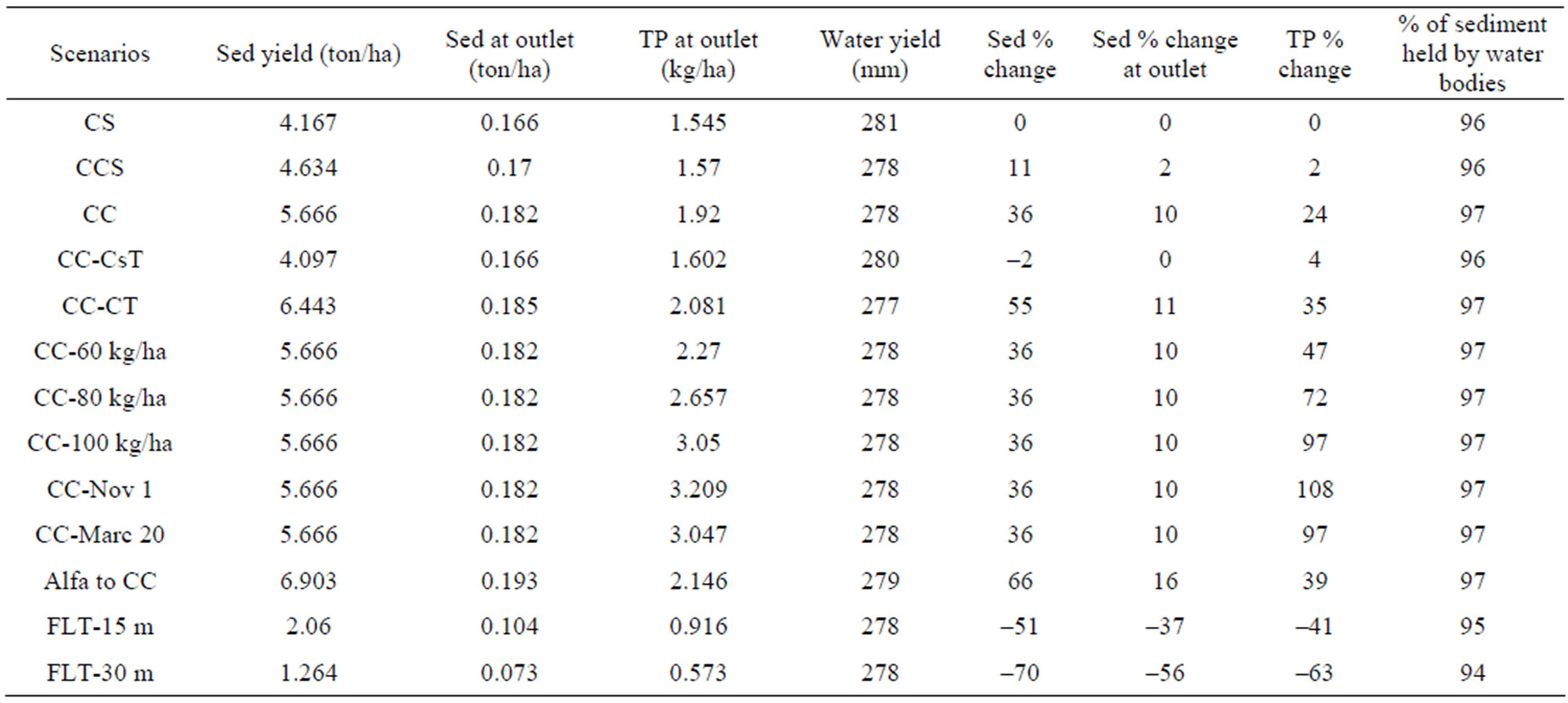
Table 3. Annual average results from crop management alternative scenarios.
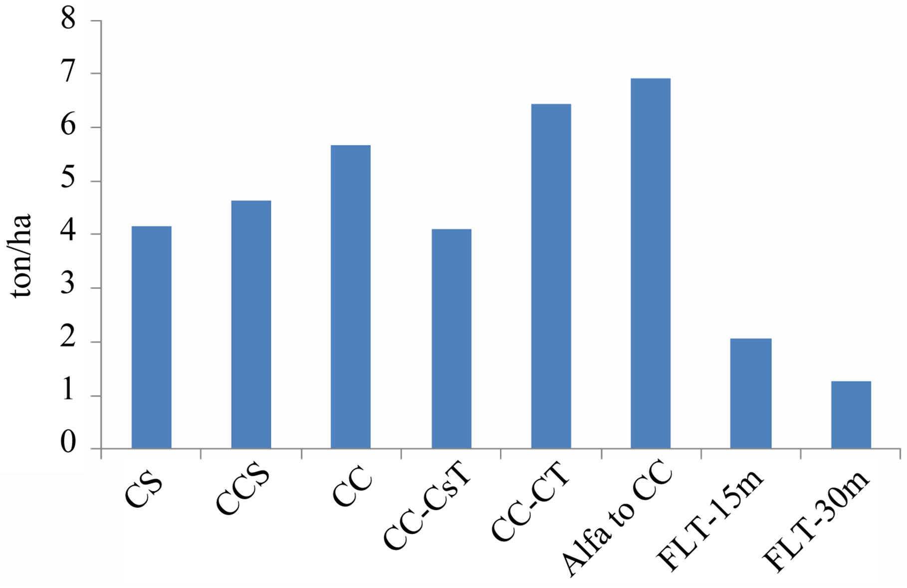
Figure 2. Annual average sediment yield from fields for crop management alternative scenarios.
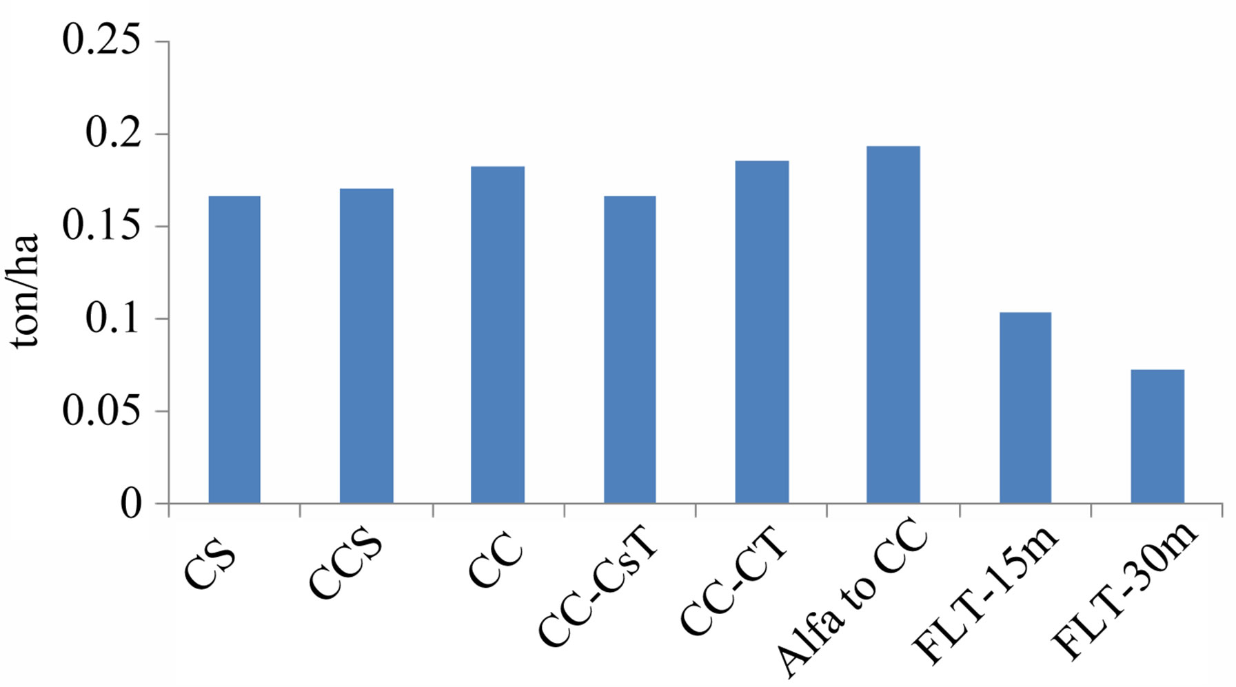
Figure 3. Annual average sediment loss at watershed outlet for crop management alternative scenarios.
caused the highest water quality damage with a 55% increase in sediment yield and 11% increase in sediment loss at the watershed outlet. Further increase in corn production by turning 7.5% of watershed area used to growth alfalfa into continuous corn produced 66% more sediment yield than the baseline and 16% more sediment loss at the watershed outlet. This large increase is because alfalfa, a perennial legume, does not require tillage every year and has deep roots that strengthen the soil structure against erosion. Scenarios with vegetative strips showed that addition of vegetative filter strips at the edge of corn fields reduced sediment loss significantly. Filter strips, 15 m and 30 m wide, reduced sediment yield by 51% and 70%, respectively. A 37% and 56% reduction in sediment loss was observed at the watershed outlet for 15 m and 30 m filter strips, respectively. Total phosphorus (TP) loss results are depicted in Table 3 and Figure 4. The conversion of corn-soybean land use to two-year corn and third year soybean increased TP loss by 2% from a base year TP loss of 1.55 kg/ha. The conversion of corn-soybean land use to continuous corn caused a 4% increase in TP loss when generic conservation tillage was used, 24% increase when reduced tillage was used, and 35% increase when conventional tillage was used (Table 3). Normally, phosphorus is bound to soil particles and loss of sediment results in loss of TP. However, during transport in water bodies a portion of TP dissolves in water and this explains higher TP increase than sediment increase at the watershed outlet after the majority of sediment settled in water bodies. Results also indicated a greater TP loss with increases in fertilization rate. When fertilization rate was increased from 41 kg/ha to 60, 80 and 100 kg/ha, TP loss increased 47%, 72% and 97%, respectively. Also, the time of fertilizer application had an impact on TP loss. When 100 kg/ha was applied on November 1st the year previous to planting then TP loss was 108% higher for continuous corn than the TP of the base year (corn-soybean). The fertilizer applied on March 20th and April 20th close to planting did not show significant difference in TP loss. This implies that the application of phosphorus in fall prior to planting is not advisable since P transport due to water runoff is high during non-growth period. When the alfalfa land use (7.5% of watershed area) was also converted to continuous corn there was 39% higher TP loss than the base year for a 41 kg/ha corn P fertilization rate. Perennial legumes, such as alfalfa, require minimal amount of P fertilizer compared to corn and as mentioned earlier, alfalfa increases resistance to transport of sediment which reduces TP loss because P bound on soil particles. Results for continuous corn (with a 100 kg/ha P fertilization rate) protected with 15 m and 30 m wide vegetative filter showed a 41% and 63% reduction in TP loss, respectively. Roots of grass and plant used for filter strips promotes infiltration which reduce surface runoff, strengthens soil from erosion, and uptake nutrients from loss. The change of land use from corn-soybean to continuous corn did not have a significant impact on water yield (only 1% reduction) in this study. Monthly loss of sediment and TP at the watershed outlet from various crop management alternatives (Figures 5 and 6) showed that continuous corn (alfalfa into corn also) had the highest sediment loss and 30 m filter strip scenario had the lowest sediment loss in the period of planting. During plant growth period, there was lower sediment loss as shown in Figure 5 and all scenarios showed roughly similar sediment loss except scenarios that have filter strips that reduced sediment. TP loss was also reduced during plant growth period as shown on Figure 6 and the difference between scenarios was smaller. However, vegetative buffer strips reduced TP significantly throughout the year. It was also noticed that monthly sediment and TP loss follows the trend of surface runoff as shown on Figures 5 and 6.
4. Discussion and Conclusion
The results in this study are in agreement with previous studies [11-13,15] that also demonstrated that implementation of best management practices could reduce increase in TP and sediment loss caused by land use
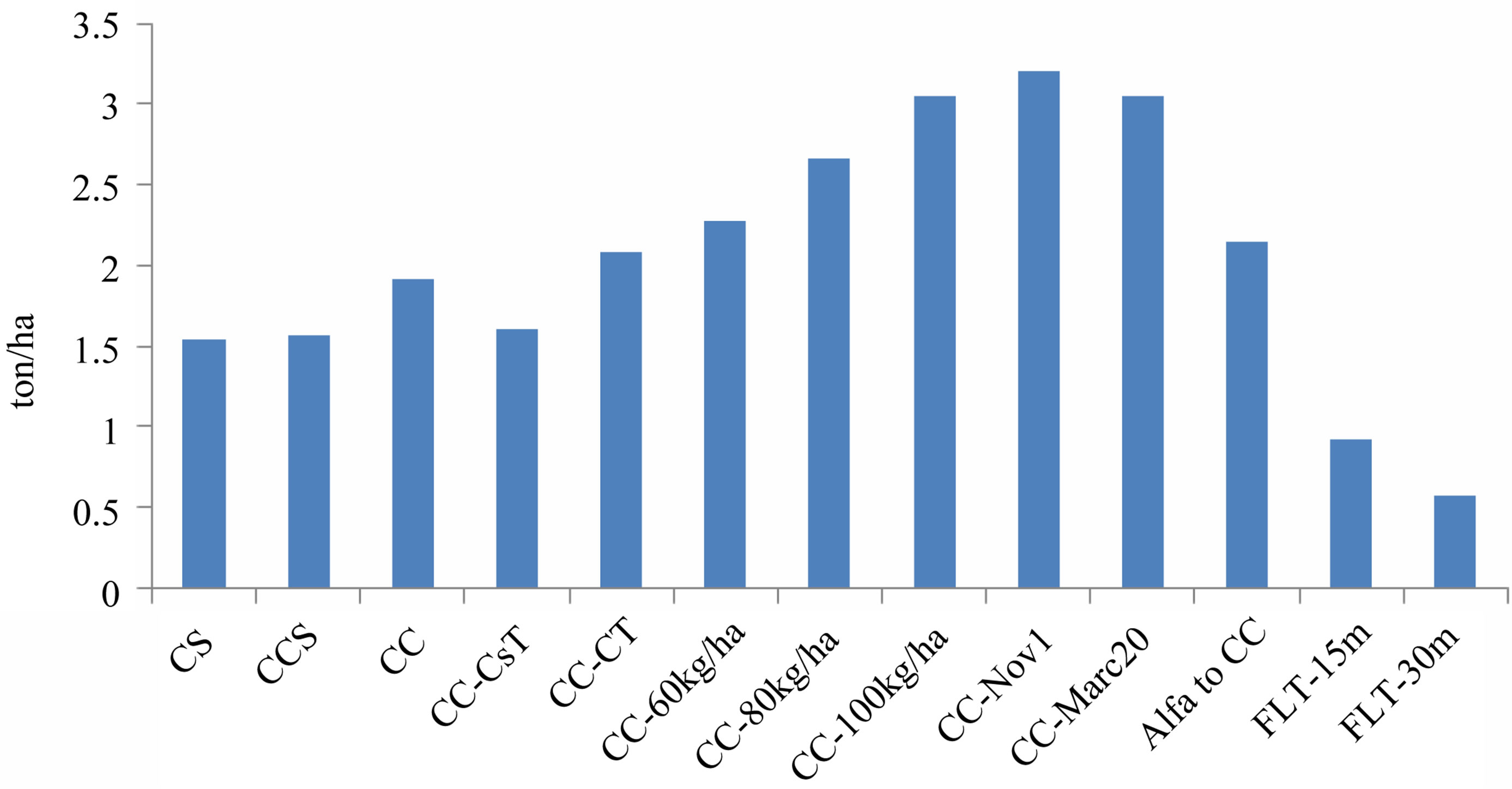
Figure 4. Annual average TP loss at watershed outlet for crop management alternative scenarios.
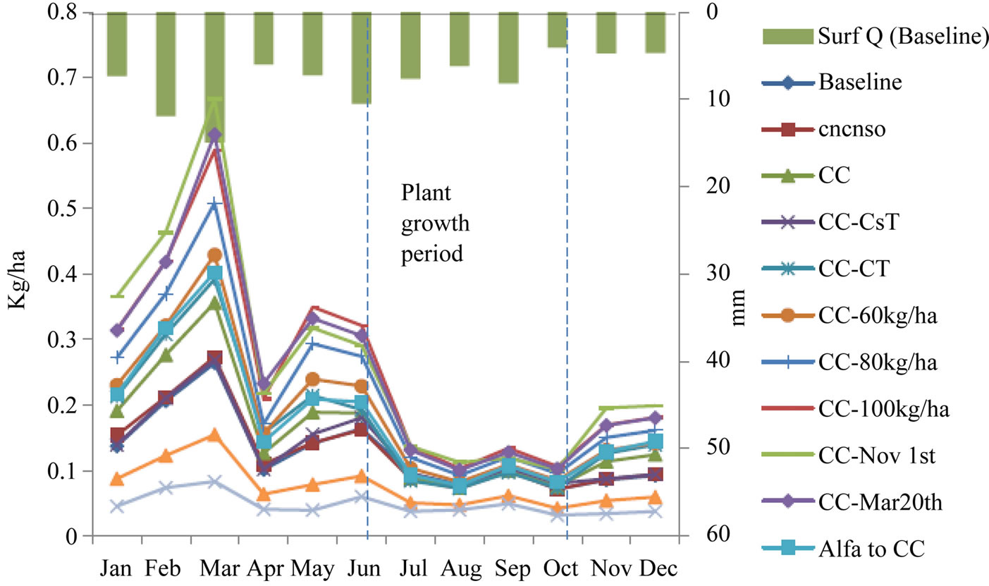
Figure 5. Monthly average sediment loss at the watershed outlet from different crop management alternative scenarios.
Figure 6. Monthly average TP loss at the watershed outlet from different crop management alternative scenarios.
change. Application of proper fertilization rates, conservation tillage and vegetative strips were shown as effective BMPs to mitigate sediment and TP loss increase when corn-soybean rotation and alfalfa farmlands were progressively converted into continuous corn for biofuel generation. Results also indicated that, for watersheds with reservoirs along the main channel, sediments loads at the watershed outlet did not vary significantly with land use change. The comparison between SWAT model output sediment yield from fields and output at the watershed outlet indicated that the majority of sediment is retained by water bodies or reservoirs. The increase in sediment and TP loss could lead to a reduction of these water bodies’ depth and eutrophication. The next issue which is beyond the objective of this study is the cost, acceptability and feasibility of BMPs in the study region. Previous studies showed that frequent testing of soil P could be used to promote optimization of P fertilizer for farmers who use excessive fertilizers. Since residue left by conservation tillage and no till could affect yield for poorly drained soils, identification of poorly and well drained soils could help determine suitable area for implementation of conservation tillage. Even though implementation of vegetative buffer strips could be costlier than other BMPs, they were shown to be most effective at reducing sediment and phosphorus loss in this study. This study also showed that SWAT model is an important tool for decision making on BMPs. However it lacks the ability to simulate some particular conservation tillage methods such as ridge till, which creates raised planting berm by tilling strips 13 to 23 cm deep and 15 to 26 cm wide, and leaves the soil and residue undisturbed between the tilled zones. In addition, SWAT does not have the ability to simulate application of fertilizer in bands where crops are planted.
5. Acknowledgements
The authors are grateful for reviewers who provided many valuable comments to improve the manuscript. Although this work was reviewed by USEPA and approved for publication; it may not necessarily reflect official Agency policy. Mention of trade names or commercial products does not constitute endorsement or recommendation for use.
REFERENCES
- R. B. Alexander, R. Smith, G. Schwarz, E. Boyer, J. Nlan and J. Brakebill, “Differences in Phosphorus and Nitrogen Delivery to the Gulf of Mexico from the Mississippi River Basin,” Environmental Science & Technology, Vol. 42, No. 3, 2008, pp. 822-830. doi:10.1021/es0716103
- USEPA, “National Water Quality Inventory,” Report to Congress, 2004 Reporting Cycle.
- T. W. Simpson, R. W. Howarth, H. W. Paerl, A. Sharpley and K. Mankin, “The New Gold Rush: Fueling Ethanol Production While Protecting Water Quality,” Journal of Environmental Quality, Vol. 37, No. 2, 2008, pp. 318-324. doi:10.2134/jeq2007.0599
- D. A. Landis, M. M. Gardiner, W. Van der Werf and S. Swinton, “Increasing Corn for Biofuel Production Reduces Biocontrol Services in Agricultural Landscapes,” Proceedings of the National Academy of Sciences of the United States of America, Vol. 105, No. 51, 2008, pp. 20552-20557. doi:10.1073/pnas.0804951106
- The CADMUS Group, Inc., “Total Maximum Daily Loading (TMDL) for Total Phosphorus and Total Suspended Solids in the Rock River Basin,” Final Report, July 2011.
- A. N. Sharpley, B. Foy and P. Withers, “Practical and Innovative Measures for Control of Agricultural Phosphorus Losses to Water: An Overview,” Journal of Environmental Quality, Vol. 29, No. 1, 2000, pp. 1-9. doi:10.2134/jeq2000.00472425002900010001x
- M. W. Gitau, W. J. Gburek and A. R. Jarrett, “A Tool for Estimating BMP Effectiveness for Phosphorus Pollution Control,” Journal of Soil and Water Conservation, Vol. 60, No. 1, 2005, pp. 1-10.
- A. N. Sharpley and H. Tunney, “Phosphorous Research Strategies to Meet Agricultural and Environmental Challenges of the 21st Century,” Journal of Environmental Quality, Vol. 29, No. 1, 2000, pp. 176-181. doi:10.2134/jeq2000.00472425002900010022x
- Y. Yuan, R. L. Bingner and R. A. Rebich, “Evaluation of AnnAGNPS on Mississippi Delta MSEA Watersheds,” Transactions of the ASAE, Vol. 44, No. 5, 2001, pp. 1183-1190.
- L. Heathwaite, A. Sharpley and W. Gburek, “A Conceptual Approach for Integrating Phosphorus and Nitrogen Management at Watershed Scales,” Journal of Environmental Quality, Vol. 29, No. 1, 2000, pp. 158-166. doi:10.2134/jeq2000.00472425002900010020x
- I. Chaubey, L. Chiang, M. W. Gitau and S. Mohamed, “Effectiveness of Best Management Practices in Improving Water Quality in Pasture-Dominated Watershed,” Journal of Soil And Water Conservation, Vol. 65, No. 6, 2010, pp. 424-437. doi:10.2489/jswc.65.6.424
- Y. Yuan, R. L. Bingner and M. A. Locke, “A Review of Effectiveness of Vegetative Buffers on Sediment Trapping in Agricultural Areas,” Ecohydrology, Vol. 2, 2009, pp. 321-336. doi:10.1002/eco.82
- Y. Yuan, M. H. Mehaffey, R. D. Lopez, R. L. Bingner, R. Bruins, C. Erickson and M. A. Jackson, “AnnAGNPS Model Application for Nitrogen Loading Assessment for the Future Midwest Landscape Study,” Water, Vol. 3, 2011, pp. 196-216. doi:10.3390/w3010196
- G. W. Roth, “Crop Rotations and Conservation Tillage,” Conservation Tillage Series (1), College of Agricultural Sciences Cooperative Extension, Penn State University, 1996.
- W. Rawls and H. H. Richardson, “Runoff Curve Numbers for Conservation Tillage,” Journal of Soil and Water Conservation, Vo. 38, No. 6, 1983, pp. 494-496.
- J. Dejong-Hughes and J. Vetsch, “On-Farm Comparison of Conservation Tillage Systems for Corn Following Soybeans,” University of Minnesota Extension, 2007.
- J. G. Arnold, R. Srinivasan, R. S. Muttiah and J. R. Williams, “Large Area Hydrologic Modeling and Assessment, Part I: Model Development,” Journal of American Water Resources Association, Vol. 34, No. l, 1998, pp. 73-89. doi:10.1111/j.1752-1688.1998.tb05961.x
- S. L. Neitch, J. G. Arnold, J. R. Kiniry and J. R. Williams, “Soil and Water Assessment Tool Theoretical Documentation,” Blackland Research Center, Temple, Texas, 2005.
- B. Schmalz and N. Fohrer, “Comparing Model Sensitivities of Different Landscapes Using the Ecohydrological SWAT Model,” Advances in Geosciences, Vol. 21, 2009, pp. 91-98. doi:10.5194/adgeo-21-91-2009
- M. W. Gitau, L. Chiang, M. Sayeed and I. Chaubey, “Watershed Modeling Using Large-Scale Distributed Computing in Condor and SWAT,” Simulation, Vol. 88, No. 3, 2012, pp. 365-380. doi:10.1177/0037549711402524
- M. Mehaffey, R. Van Remortel, E. Smith and R. Bruins, “Developing a Dataset to Assess Ecosystem Services in the Midwest United States,” International Journal of Geographic Information Services, Vol. 25, 2011, pp. 681- 685. doi:10.1080/13658816.2010.497148
- D. N. Moriasi, J. G. Arnold, M. W. Van Liew, R. L. Bingner, R. D. Harmel and T. L. Veith, “Model Evaluation Guidelines for Systematic Quantification of Accuracy in Watershed Simulations,” Transactions of the ASABE, Vol. 50, No. 3, 2007, pp. 885-900.
- K. L. White and I. Chaubey, “Sensitivity Analysis, Calibration, and Validation for a Multisite and Multivariable SWAT Model,” Journal of the American Water Resources Association, Vol. 41, No. 5, 2005, pp. 1077-1089. doi:10.1111/j.1752-1688.2005.tb03786.x
- P. W. Gassman, M. R. Reyes, C. H. Green and J. G. Arnold, “The Soil and Water Assessment Tool: Historical Development, Application and Future Research Directions,” Transactions of ASABE, Vol. 50, No. 4, 2007, pp. 1211-1250.
- A. Van Griensven, T. Meixner, S. Grunwald, T. Bishop, M. Di Luzio and R. A. Srinivasan, “Global Sensitivity Analysis Method for the Parameters of Multi-Variable Watershed Models,” Journal of Hydrology, Vol. 324, No. 1-4, 2006, pp. 10-23. doi:10.1016/j.jhydrol.2005.09.008
- USDA-NRCS, “Rusle 2 and Crop Management Zones,” 2011. http://fargo.nserl.purdue.edu/rusle2_dataweb/RUSLE2_Index.htm
- S. L. Neitch, J. G. Arnold, J. R. Kiniry and J. R. Williams, “Soil and Water Assessment Tool Input/Output File Documentation,” Blackland Research Center, Temple, Texas, 2005.
- J. B. Peters, C. A. M. Laboski and L. G. Bundy, “Sampling Soils for Testing,” University of Wisconsin-Extension Publication A2100, 2007.