Journal of Water Resource and Protection
Vol.4 No.3(2012), Article ID:17945,12 pages DOI:10.4236/jwarp.2012.43014
Particle Swarm Optimization for Identifying Rainfall-Runoff Relationships
Department of Design for Sustainable Environment, Ming Dao University, Changhua, Chinese Taipei
Email: jamin@mdu.edu.tw
Received January 2, 2012; revised February 7, 2012; accepted March 4, 2012
Keywords: Rainfall-Runoff; System Identification; Particle Swarm Optimization; Classic Models; Simple Linear Model
ABSTRACT
Rainfall-runoff processes can be considered a single input-output system where the observed rainfall and runoff are inputs and outputs, respectively. Conventional models of these processes cannot simultaneously identify unknown structures of the system and estimate unknown parameters. This study applied a combinational optimization and Particle Swarm Optimization (PSO) for simultaneous identification of system structure and parameters of the rainfall-runoff relationship. Subsystems in proposed model are modeled using combinations of classic models. Classic models are used to transform the system structure identification problem into a combinational optimization and can be selected from those typically used in the hydrological field. A PSO is then applied to select the optimized subsystem model with the best data fit. The parameters are estimated simultaneously. The proposed model is tested in a case study of daily rainfall-runoff for the upstream Kee-Lung River. Comparison of the proposed method with simple linear model (SLM) shows that, in both calibration and validation, the PSO simulates the time of peak arrival more accurately compared to the SLM. Analytical results also confirm that the PSO accurately identifies the system structure and parameters of the rainfall-runoff relationship, which are a useful reference for water resource planning and application.
1. Introduction
The rainfall-runoff process in a river basin can be conceptualized as a single input-output system. When modeling such a system, the goal is to use historic data for predicting further runoff by analyzing the input-output relationship based on observed input-output data, i.e., system identification. The “black-box” approach emphasizes system functions rather than system characteristics or natural laws governing the system. The system response function analyzes the black-box relationships between inputs and outputs, i.e., the system characteristics or natural laws governing system operation. The system response function also varies according to system characteristics or according to natural laws. In black-box models, the task is describing or approximating the system response function.
The identifications and applications of hydrological black-box models have been thoroughly investigated. Cheng et al. [1] presented an automatic calibration methodology, which consists of water balance parameter and runoff routing parameter calibration, for Xinanjiang model. Their results showed that the hybrid methodology of genetic algorithms (GAs) and the fuzzy optimal model (FOM) is not only capable of exploiting more the important characteristics of floods but also efficient and robust. Chau et al. [2] employed the GA-based artificial neural network (ANN-GA) and the adaptive-network-based fuzzy inference system (ANFIS) for flood forecasting in a channel reach of the Yangtze River in China. They found that the ANFIS model is optimal and the performance of the ANN-GA model is also good.
Lin et al. [3] considered the support vector machine (SVM) as a promising method for hydrological prediction. In their study, the SVM prediction model was tested using the long-term observations of discharges of monthly river flow discharges in the Manwan Hydropower Scheme. Through the comparison of its performance with those of the autoregressive moving-average (ARMA) and ANN models, it is demonstrated that SVM is a very potential candidate for the prediction of longterm discharges. Cheng et al. [4] explored a novel chaos GA (CGA) based on the chaos optimization algorithm (COA) and GA to overcome premature local optimum and increase the convergence speed of GA. Their results showed that the long term average annual energy based CGA is the best and its convergent speed not only is faster than dynamic programming largely, but also overpasses the standard GA. Thus, their proposed approach was feasible and effective in optimal operations of complex reservoir systems.
Wang et al. [5] examined ARMA models, ANNs approaches, adaptive neural-based fuzzy inference system (ANFIS) techniques, genetic programming (GP) models and SVM method using the long-term observations of monthly river discharges. They found that the best performance can be obtained by ANFIS, GP and SVM, in terms of different evaluation the training and validation phases. Wu et al. [6] proposed a crisp distributed support vectors regression (CDSVR) model for monthly streamflow prediction in comparison with four other models: ARMA, K-nearest neighbors (KNN), ANNs, and crisp distributed ANNs (CDANNs). Their results showed that models fed by preprocessed data perform better than models fed by original data, and CDSVR outperform other models except for at a 6-month-ahead horizon for Danjiangkou. They also found that the performance of CDSVR deteriorated with the increase of the forecast horizon.
Hydrological models such as simple linear model (SLM) are suitable for hydrological system identification because they can simply and conventionally estimate total runoff from total rainfall. However, conventional models for performing the above system identification are limited because they cannot simultaneously identify the unknown structure of the system and estimate unknown parameters. Wang et al. [7] developed a new method of using Particle Swarm Optimization (PSO) algorithm for system identification. Its novel feature is the use of classic models to transform the system structure identification problem into a combinational problem. A PSO algorithm is then used to identify system structure and parameters. This study applies the concept developed by Wang et al. [7] to model the rainfall-runoff relationship.
Kennedy and Eberhart [8] originally developed the PSO algorithm for a simplified simulation of animal social behaviors. The PSO, which is a population-based and self-adaptive search optimization technique, is now widely used to solve discrete and continuous optimization problems. Recently, PSO has been employed extensively in hydrological forecasting and water resources management. Chau [9] developed a PSO model for training perceptions in ANNs. Applications of PSO predicting water levels show that the technique is an effecttive alternative algorithm for training ANNs.
Gill et al. [10] introduced PSO, a relatively new global optimization tool that has already proven effective and efficient in various fields. Although PSO initially had a single-objective function, the approach has been extended to deal with multiple objectives in a form called multiobjective PSO (MOPSO). Tests of this approach for parameter estimation of a well-known 13-parameter conceptual rainfall-runoff model of Sacramento soil moisture show very encouraging modeling results. Chau [11] developed and applied a split-step PSO model to train multi-layer perceptions for forecasting real-time water levels. This paradigm combines the advantages of the global search capability of PSO algorithm in the first step with fast local convergence of Levenberg-Marquardt algorithm in the second step. Performance comparisons show that its speed and accuracy are better than those of the benchmarking backward propagation algorithm and the standard PSO algorithm.
Luo and Yuan [12] used PSO to optimize an integrated water system by combining water usage processes and water treatment operations into a single network such that the total cost of fresh water and wastewater treatment is florally minimized. Zhang et al. [13] tested five global optimization algorithms (GAs, shuffled complex evolution, PSO, differential evolution, and artificial immune system) for automatic parameter calibration in a complex hydrologic model of four watersheds constructed using Soil and Water Assessment Tool (SWAT). The results show that GA outperform the other four algorithms when more than 2000 models are analyzed while PSO obtains better parameter solutions when fewer than 2000 models are run. The PSO algorithm is preferable when computation time is limited whereas GA is preferable when substantial computational resources are available. When applying both GA and PSO for optimizing SWAT parameters, the population size should be small.
In a SVM developed by Wang et al. [14] for forecasting annual reservoir inflow, PSO is used for parameter optimization. For the data set used in that study, the SVM model outperformed the ANN models in terms of forecasting performance. Gaur et al. [15] applied Analytic Element Method (AEM) in a PSO-based simulation-optimization model of groundwater management problems. The AEM-PSO model proved efficient for optimizing the location and discharge of pumping wells. The penalty function approach was also effective when using PSO to solve groundwater hydraulic management problems.
In conventional procedure for performing system identification, after determining system structures, the optimization method can be then adopted to parameter estimation. However, it is difficult to identify system structures. This work employs classic models to transform the system structure identification problem into a combinational optimization problem. The proposed method can simultaneously identify unknown structures of the system and estimate unknown parameters. Firstly, the subsystem models include a combination of classic models that can be selected from those models typically used in the hydrological field. The PSO is then used for simultaneous identification of the system structure and parameters. The rest of this paper is organized as follows. First, the concept of system identification and the SLM structures are described. The PSO algorithm and its implementation procedure are then defined. Next the efficacy of the proposed method is demonstrated in a case study of a small Taiwan watershed. Finally, analytical results are discussed, and conclusions are given.
2. System Identification
2.1. The Description of System Identification
A system can be identified from observed input and output data to obtain the equivalent system. The purpose of system identification is to understand variation in the system so that the identified results can be applied to solving practical problems. The system identification in this study is the method that selects the combination of the subsystem model that best fits the sample data from many subsystems and estimates their parameters. Classic models are used to transform the system structure identification problem into a combinational optimization problem. The system model consists of subsystem models that are the combination of classic models. Classic models can be selected from models typically used in the hydrological field. The principles of selecting classic models are general, classic and includable [7].
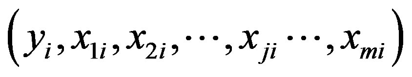
Consider a static system with multiple inputs and single output. Suppose that y is the output of an observable system affected by m input, i.e., x1, x2,···, xm. The n groups of observed data can be described as follows [7]:
 (1)
(1)
where xji is the j-th input data of group i, yi is the output data of group i, i = 1, 2,···, n; j = 1, 2,···, m.
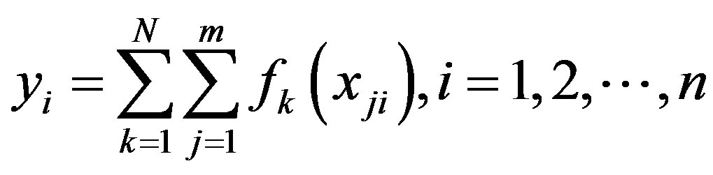
Suppose that the observed data include various possible subsystem models that are combinations of classic models. Classic models can be selected from the models that usually appear in the hydrological field. Now consider the case where single variable xj affects the output of system by the form of f(xj). The f(xj) is then defined as a classic model with a single variable [7]. Let N be the total number of classic models with a single variable. The output, which is affected by various input data, can be expressed as [7]
 (2)
(2)
2.2. The Simple Linear Model
The simple and conventional method used to estimate the system response function from rainfall-runoff data is the SLM [16]. The SLM is compared with the proposed method in this study.
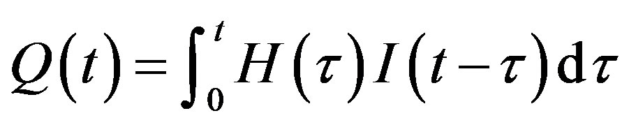
Let I(t) and Q(t) represent total rainfall and total runoff of a watershed, respectively, and let H(t) represent the system response function. The rainfall-runoff process is assumed to be a linear, time-invariant, and single inputoutput system. The function of the SLM system can be represented by a linear convolution equation as follows [16]:
 (3)
(3)
where τ is an integral variable.
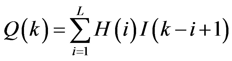
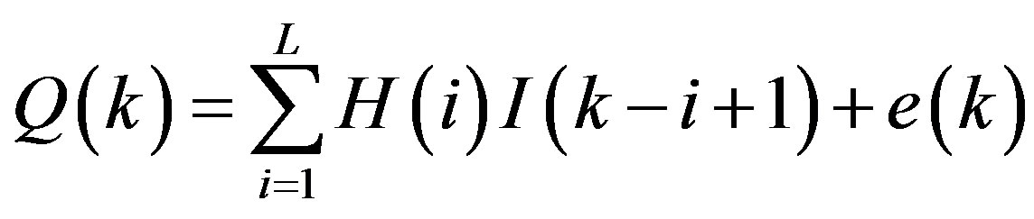
Equation (3) can be applied in discrete form as follows [16]:
 (4)
(4)
where L is the memory length of a watershed, I(k – i + 1) is the average rainfall at time k – i + 1, Q(k) is the total runoff at time k, H(i) is a system response function.
Equation (5) reveals data error or incomplete assumptions about linearity [16]:
 (5)
(5)
where e(k) is a random error term.
Equation (5) can be expressed using matrix equations as follows [16]:
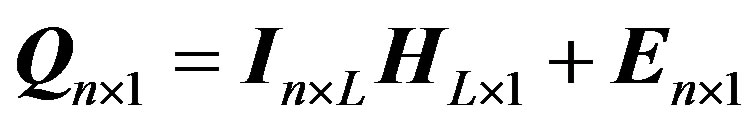 (6)
(6)
where n is the total length of hydrological data, and L is the memory length of a system response function.
The system response function H can be identified by Least Squares (LS) method. The essential principle of LS is to minimize the sum of squares of the differences between the observed and estimated values. The objective function is defined as follows [16]:
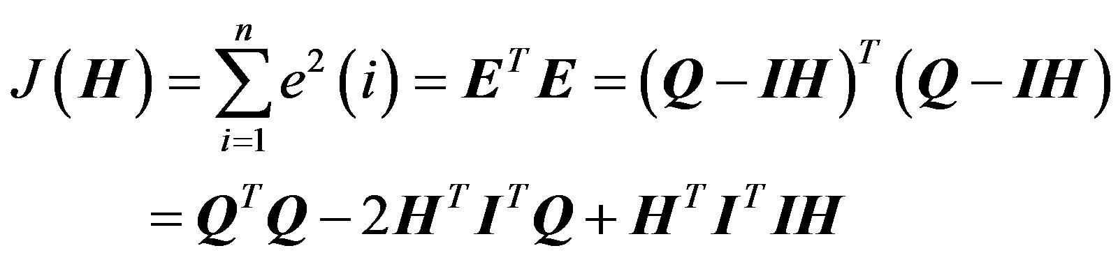 (7)
(7)
The system response function can be derived by minimizing the objective function, i.e., min as shown below [16].
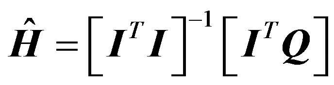 (8)
(8)
3. Particle Swarm Optimization
The PSO, which was introduced by Kennedy and Eberhart in 1995 and known as an optimizer, is an approach to optimize information flow without complex operators. The PSO adopts the current optimal solution as the mechanism for renewing the whole search process such that the PSO is capable of rapid convergence to a reasonably good solution.
3.1. Underlying Theory of PSO
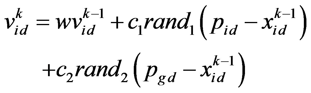
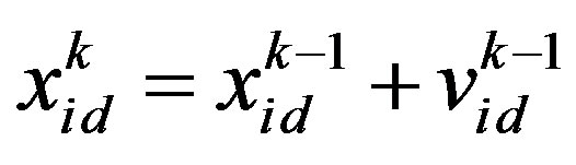
In PSO, several particles (M particles) are denoted as the potential solution flying in the problem search space to locate their optimum positions. Each particle is represented by a vector in multidimensional space D. Assume the position vector and velocity vector of particle i are Xi = (xi1, xi2,···, xid) and Vi =(vi1, vi2,···, vid), respectively. Set pi = (pi1, pi2,···, pid), i.e., pbest, as the current optimal position searched by each particle, and set gbest as the current optimal position searched by all particles of the group. For each generation, the updated equations of particle velocity and position in dimension d are as follows [17]:
 (9)
(9)
 (10)
(10)
where w is the inertia weight coefficient, c1 and c2 are acceleration coefficients, rand1 and rand2 are random numbers in the interval [0,1], and i = 1, 2,···, M. The  is the component of fly velocity vector of particle i in dimension d for generation k. The
  is the component of position vector of particle i in dimension d for generation k. The pid is the component of the current optimal position vector pbesti searched by particle i in dimension d. The pgd is the component of the current optimal position vector gbest searched by all particles of the group in dimension d.
3.2. Algorithm Procedure
The procedure for performing the PSO algorithm is as follows [18].
1) Randomly generate both the position and velocity of the particle in the initial swarm for D-dimensional space.
2) Evaluate the fitness value of the particle, which is usually defined as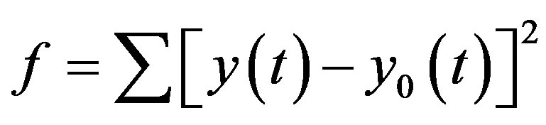 where y(t) and y0(t) are the estimated and observed output, respectively.
3) Compare the fitness value of the particle with that of the previous optimal value, and modify the new velocity of the particle according to the best positions of the particle (pbest) and swarm (gbest).
4) Compare the fitness of the particle and swarm. If the best fitness of the particle is superior to that of the swarm, modify the memory of the best fitness (gbest) value for the swarm. At the same time, every particle should modify the velocity of the particle in the next generation.
5) Determine the new velocities and positions of the particles for the next generation according to Equations (9) and (10).
6) Stop the search when the termination condition is satisfied; otherwise, return to step 2). The algorithm usually stops when the generation reaches the maximum.
4. Application and Analysis
4.1. The Proposed Method
Consider the three classic models for the relationship between rainfall input x and runoff output y, which is an example of a typical relationship in a hydrological system:
 (11)
(11)
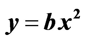 (12)
(12)
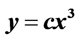 (13)
(13)
where a, b and c are constant coefficients. The input used when testing the proposed PSO method is the daily rainfall for the current day and the previous 7 days. The choice of the particular set of parameters is based on the memory length of a watershed. In addition, more parameters are included because of carrying out the combinational optimization. The daily runoff of current day is selected as output. To compare the proposed PSO with the SLM, the memory length of the watershed L is 8 days. Assume these eight inputs affect the output of system by the form f(xj). The n output can then be described as:
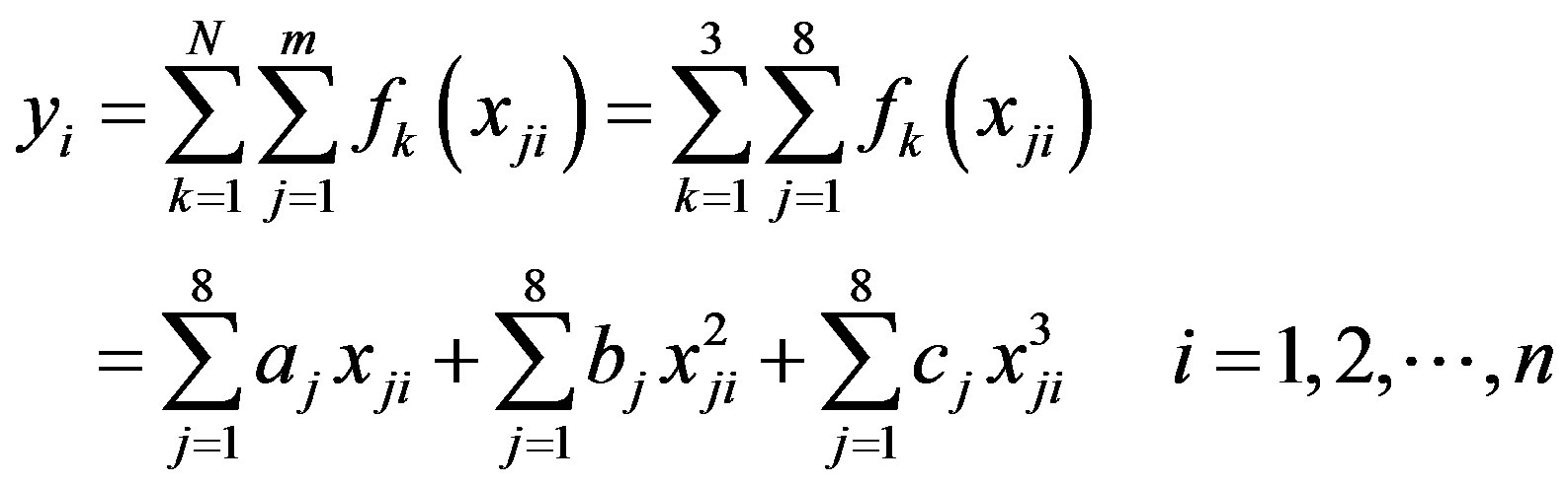 (14)
(14)
Equation (14), which includes both linear and nonlinear terms, is similar to the Volterra model typically used to identify a nonlinear system. Linear models yield fairly good results, so the effect of nonlinearity in modeling is assumed to be relatively small. Hence, Lattermann [19] considered that adding only a second term to the linear hydrological model is adequate. This investigation adopts sufficient three terms to the modeling of the nonlinear rainfall-runoff process. The coefficients of Equation (14) cannot be conveniently estimated by LS since the input matrix is singular when solving Equation (8). Some of the diagonal elements of the upper triangular matrix U of the lower and upper (LU) factorization approach zero. In this study, the PSO is applied to estimate the coefficients of Equation (14). The analytic results are compared with the results obtained using SLM.
4.2. Study Basin
This work demonstrates the feasibility of applying the proposed PSO-based method for identifying rainfallrunoff processes using the Wu-Tu watershed, which located in northern Taiwan. The watershed upstream area is 203 km2 (Figure 1). The mean annual precipitation in this watershed is 2500 mm. Due to the topography of this watershed, the runoff pathlines are short and steep, and rainfall is nonuniform in both time and space. Large floods develop quickly in the middle-to-downstream reaches of this watershed, leading to severe damage. The daily rainfall and runoff data for 1966-1994 were collected. The data for 1966-1980 were used to calibrate the proposed model, while data for 1981-1994 were used to verify the performance of the proposed method. Each year is regarded as a single event (i.e., duration is 365 days) in calibration or validation. Daily rainfall data are average values obtained from the Jui-Fang, Huo-ShaoLiao and Wu-Tu weather station using the kriging method. The daily runoff data are obtained from the Wu-Tu hydrological station.
4.3. Comparison of Model Performances
1) Coefficient of efficiency, CE, is defined as:
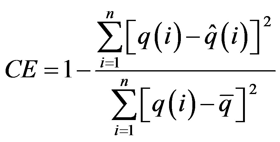 (15)
(15)
where  denotes the discharge of the simulated hydrograph for time period i (m3/s),
  is the discharge of the observed hydrograph for time period i (m3/s),
  represents the average discharge of the observed hydrograph for time period i (m3/s) and n is number of data.
The CE quantifies the goodness of fit between the estimated hydrograph and the observed hydrograph. A better fit is indicated by a CE that is closer to unity.
2) Error of Total Volume (EV)
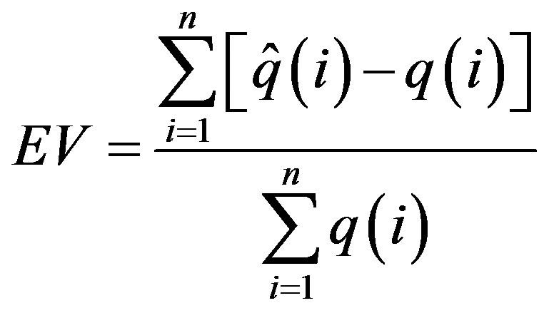 (16)
(16)
where  denotes the discharge of the simulated hydrograph for time period i (m3/s),
 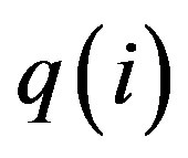 is the discharge of the observed hydrograph for time period i (m3/s). The EV specifies the mean error between the estimated hydrograph and the observed hydrograph. When the value of EV is positive, the mean estimated discharge exceeds the observed discharge, and vice versa. A better fit is represented by a smaller absolute value of EV.
3) The error of peak discharge, EQp (%), is defined as:
 (17)
(17)
where  denotes the peak discharge of the simulated hydrograph (m3/s) and qp is the peak discharge of the observed hydrograph (m3/s). When the EQp is positive, the estimated peak discharge exceeds the observed peak discharge. When EQp is negative, the estimated peak discharge is smaller than the observed peak discharge. A better fit is indicated by a smaller absolute value of EQp.
4) The error of the time for peak to arrive, ETp, is defined as:
 (18)
(18)
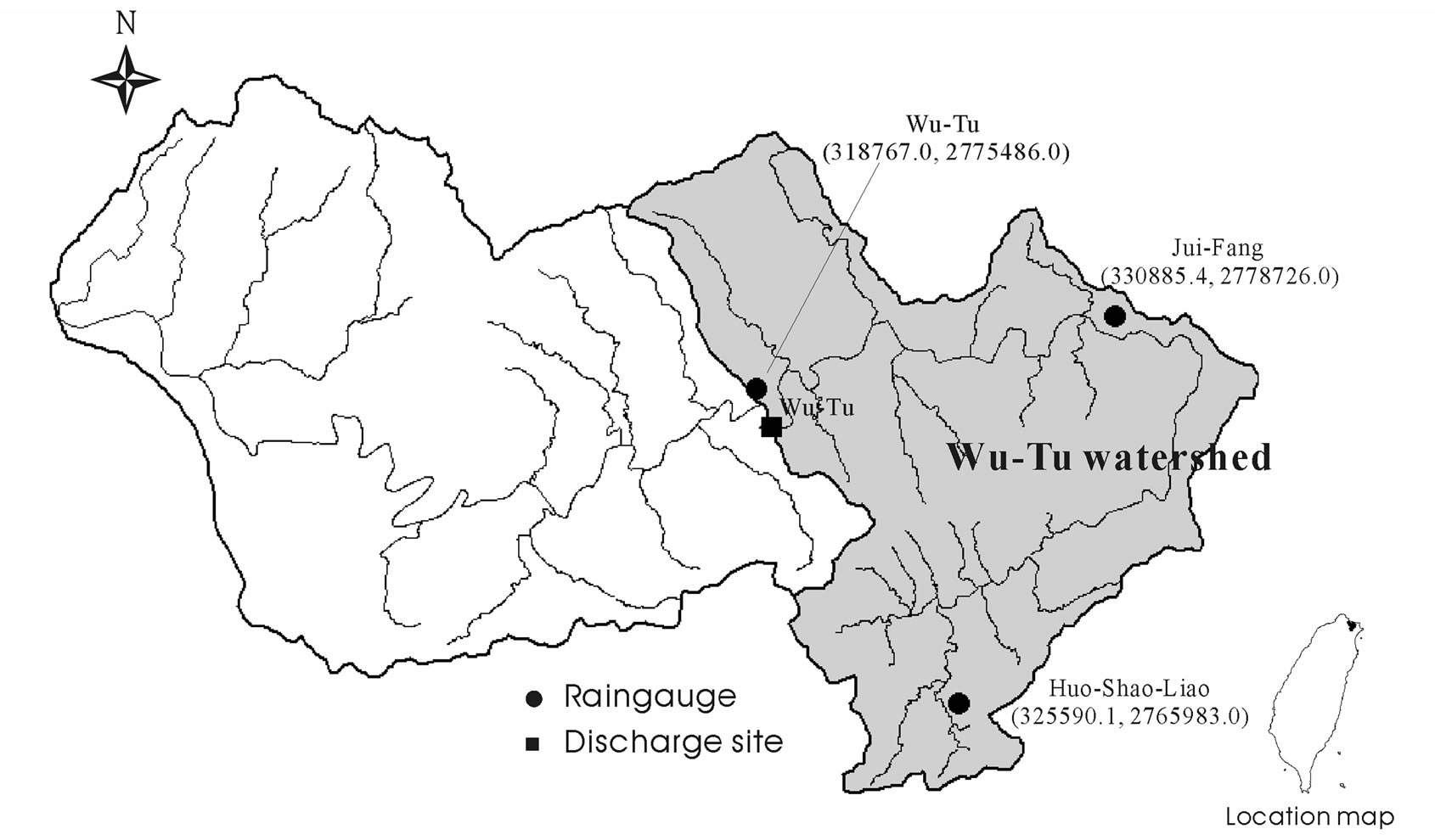
Figure 1. The map of Wu-Tu watershed showing the study area near Taipei, Taiwan.
where  denotes the time for the simulated hydrograph peak to arrive (days) and Tp represents the time required for the observed hydrograph peak to arrive (days). When ETp is negative, the estimated peak discharge precedes the observed peak discharge. When ETp is positive, the estimated peak discharge follows the observed peak discharge. A better fit is represented by a smaller absolute value of ETp.
5. Results and Discussion
The results obtained using SLM are denoted as the SLM. The results obtained using PSO in Equation (14) are denoted as the PSO. For the proposed PSO method, the total number of particle swarms, the maximum number of generations, inertia weight coefficient w, and acceleration coefficients c1 and c2 are 36, 100, 0.5, 2.0 and 2.0, respectively.
Table 1 shows the calibration results for the SLM and the PSO. Figures 2-5 display four representative calibration results. Calibration results show that the average absolute value of EV is slightly worse in the PSO (6.281%) than in the SLM (5.221%). Based on the average value of the CE criterion, the PSO (0.838) outperforms the SLM (0.827). The CE of the PSO also outperforms that of the SLM for each year. Based on the EQP criterion, the average of the absolute value of the PSO (20.701%) is slightly better than that of the SLM (21.788%). Based on the ETP criterion, the average absolute value of the PSO (3.800 days) is better than that of SLM (4.667 days). Especially in the case of year 1974 (Figure 3), the ETP of SLM is –13 days; however, the ETP of PSO is 0 days. The PSO obtains a more accurate simulation of the peak values compared to the SLM.
Table 2 presents the average value of the estimated coefficients of response function, i.e.,  , and the average value of the estimated coefficients of Equation (14), i.e.,
  ,
,  and
and , obtained from the 15 calibrated years. The average value of the estimated coefficients can be used for performance evaluations of the SLM and PSO. The average of the estimated coefficients provides not only validation data for the proposed approach, but also average system characteristics.
Table 3 shows the validation results when using SLM and PSO. Figures 6-9 display four representative validation results. Validation results demonstrate that the average absolute value of EV of the PSO (16.764%) is slightly worse than that of the SLM (15.599%). Based on the CE criterion, the PSO performs comparably to the SLM. Based on the EQP criterion, the average of the absolute value of the PSO (24.038%) is slightly worse than that of the SLM (23.735%). Based on the ETP criterion, the average of the absolute value of the PSO (15.500 days) is better than that of SLM (24.786 days). Espe-
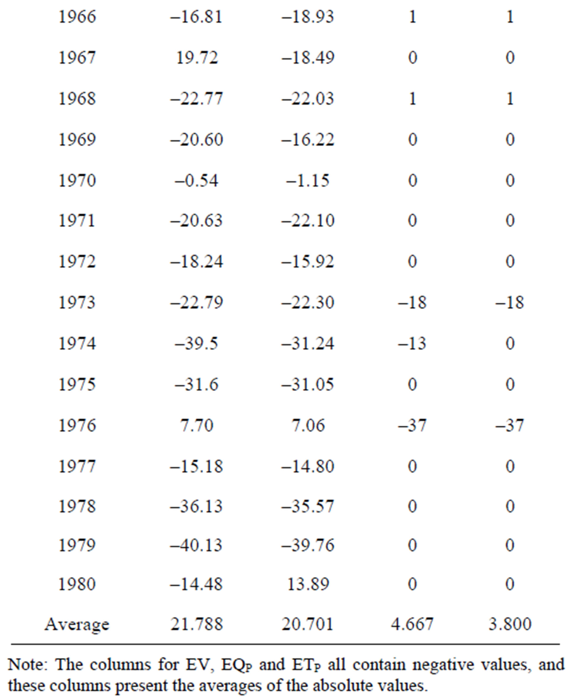
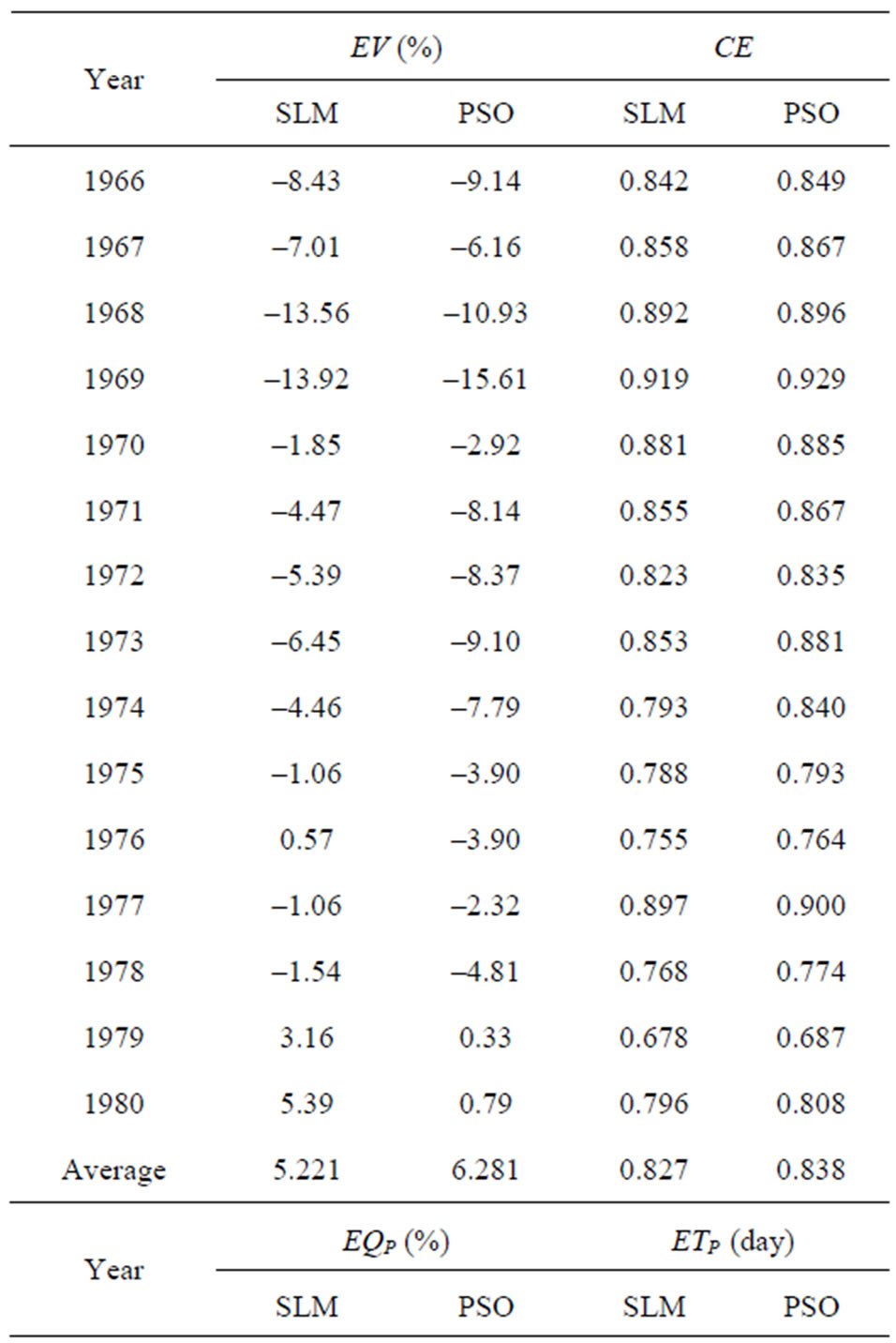
Table 1. Calibration results using SLM and PSO.
Figure 2. Calibration results using SLM and PSO (1969).
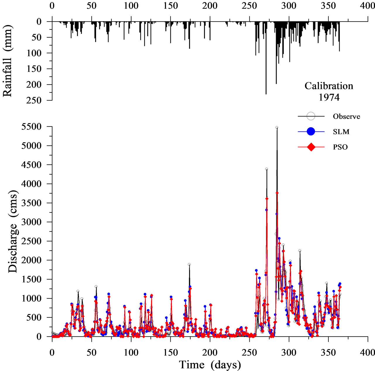
Figure 3. Calibration results using SLM and PSO (1974).
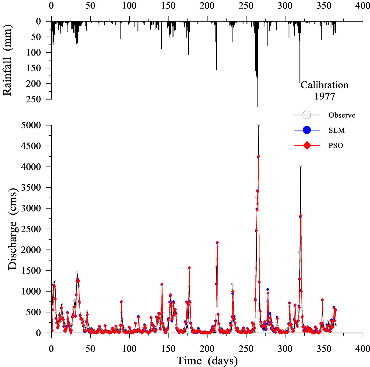
Figure 4. Calibration results using SLM and PSO (1977).
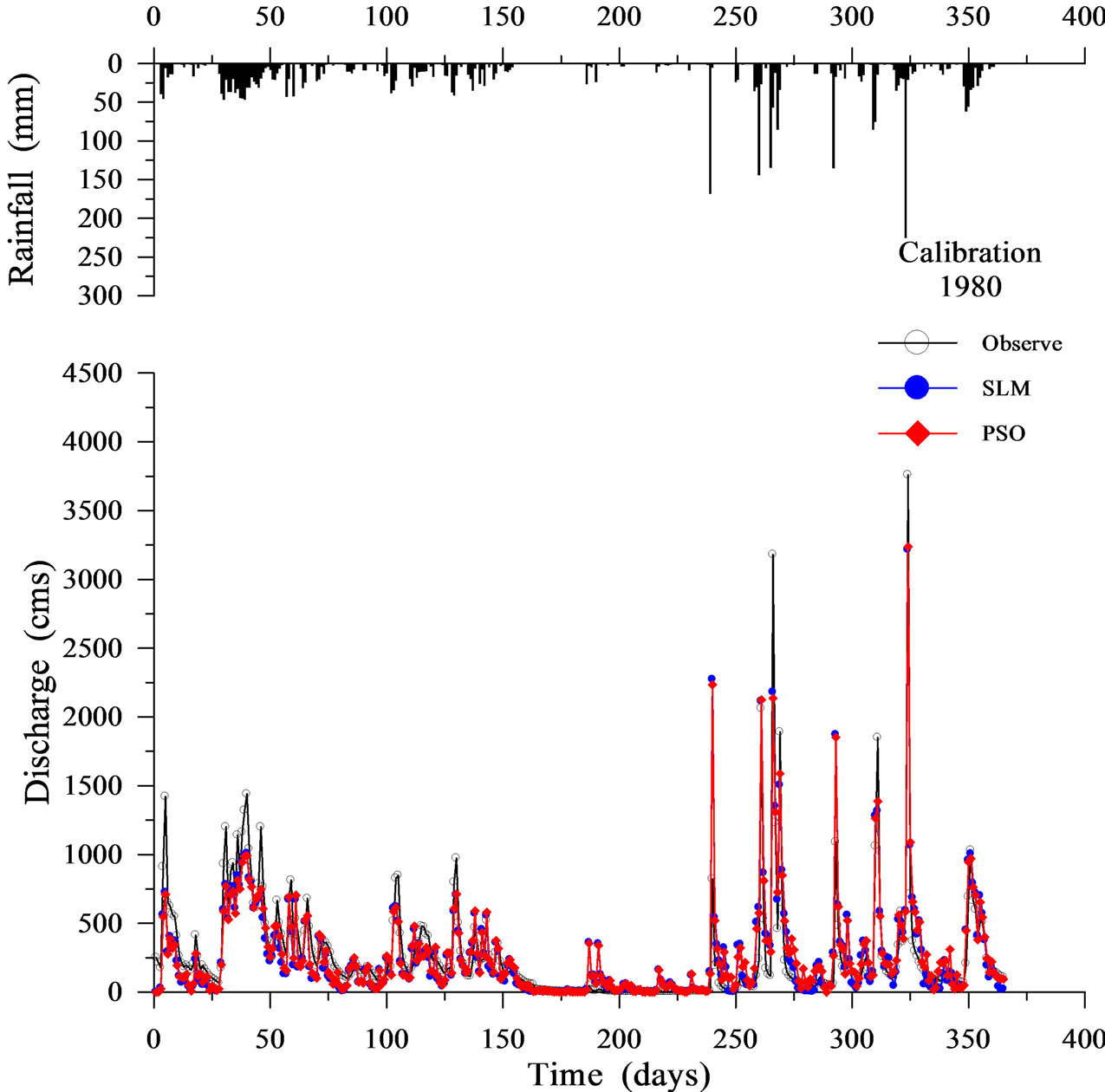
Figure 5. Calibration results using SLM and PSO (1980).
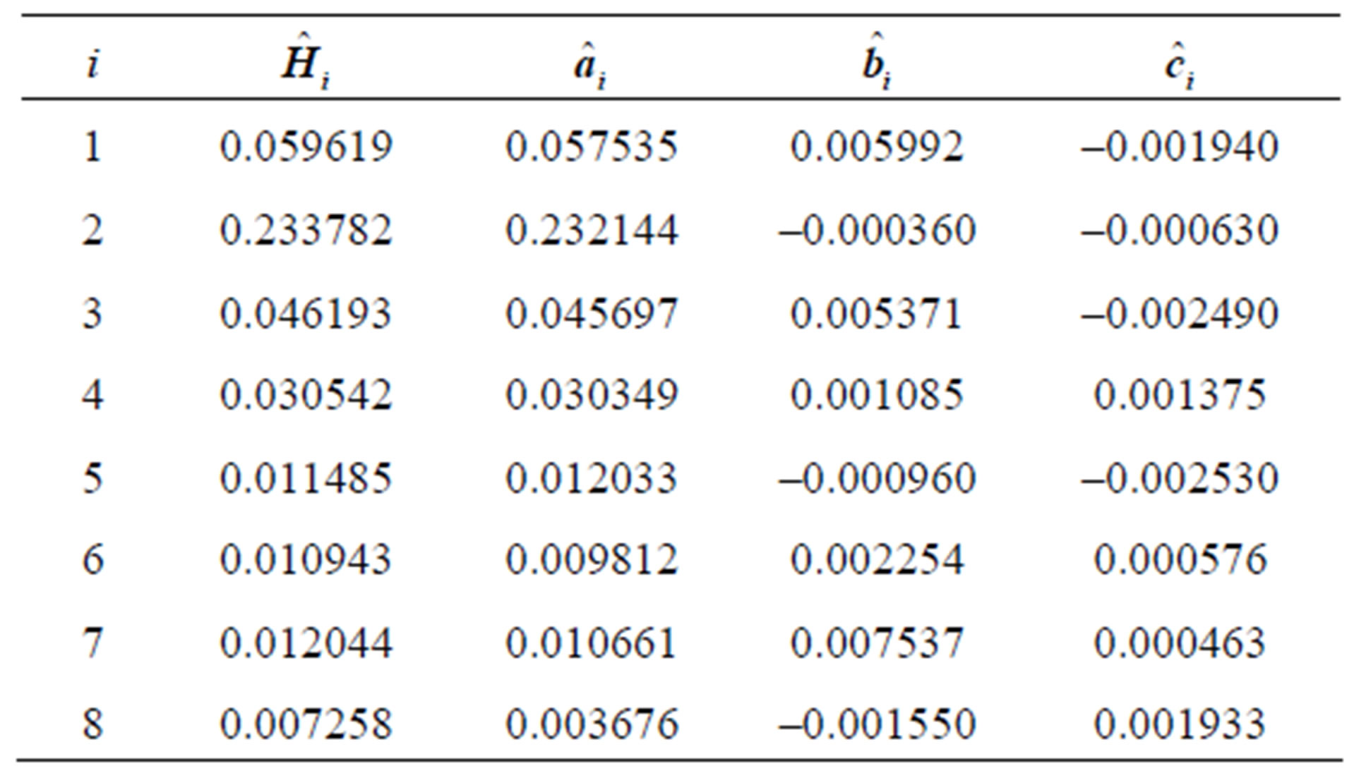
Table 2. The average estimated coefficients, obtained from the 15 calibrated events.
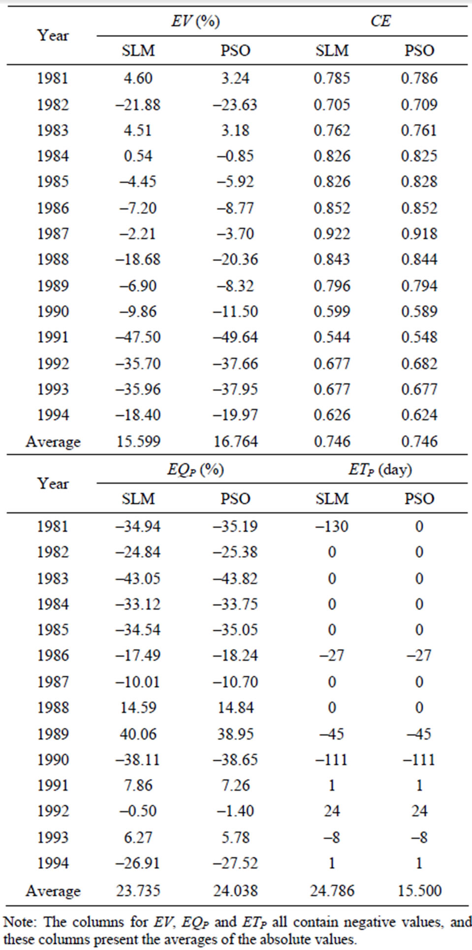
Table 3. Validation results using SLM and PSO.
cially in the case of year 1981 (Figure 6), the ETP of SLM is –130 days; however, the ETP of PSO is 0 days. The PSO can simulate the time of peak arrival more accurately compared to the SLM.
The above results can be summarized as follows. In the case of calibration results, the PSO outperforms the SLM in all criteria except EV. In terms of CE criterion in particular, the PSO outperforms the SLM in each year. These calibration results imply that the proposed PSO is suitable for identifying the rainfall-runoff relationship. In the case of validation results, the CE of the PSO is the same as that of the SLM. The PSO is slightly worse than the SLM based on the EV and EQP criteria. However, the PSO clearly outperforms the SLM based on the ETP criterion. In both the calibration and validation results, the PSO can simulate the time of peak arrival more accurately compared to the SLM. This finding apparently shows that the PSO, which includes both linear and nonlinear terms, simulates the time of peak arrival more accurately compared to the SLM, which includes only linear terms.
6. Conclusions
In this work, performance in identifying rainfall-runoff relationships was compared between PSO and conventional SLM. The calibration results for PSO are better than those of the SLM in all criteria except EV. Specifically, based on the CE criterion, the PSO outperforms the SLM in each year. The validation results for PSO are slightly worse than those for the SLM based on the EV and EQP criteria. The CE of the PSO is the same as that of the SLM. The PSO clearly outperforms the SLM based on the ETP criterion. The above results show that the proposed PSO is more suitable for modeling rainfall-runoff relationships compared to SLM.
The estimated time of peak arrival is an essential calculation. Both the calibration and validation results confirm that the PSO can simulate the time of peak arrival more accurately compared to the SLM. The main reason is that the PSO includes both linear and nonlinear terms whereas the SLM uses only linear terms.
This study applied PSO for identifying rainfall-runoff relationships. The PSO, which is a global random optimization algorithm, can simultaneously identify system structure and parameters. The daily rainfall-runoff data for the upstream Kee-Lung River are chosen to verify the appropriateness of the proposed model. Analytical results demonstrate that PSO effectively identifies the system structure and parameters of the rainfall-runoff relationship, which is an essential consideration in water resource planning and application.
The inertia weight coefficient and acceleration coefficients, which are used to adjust the velocities and posi-
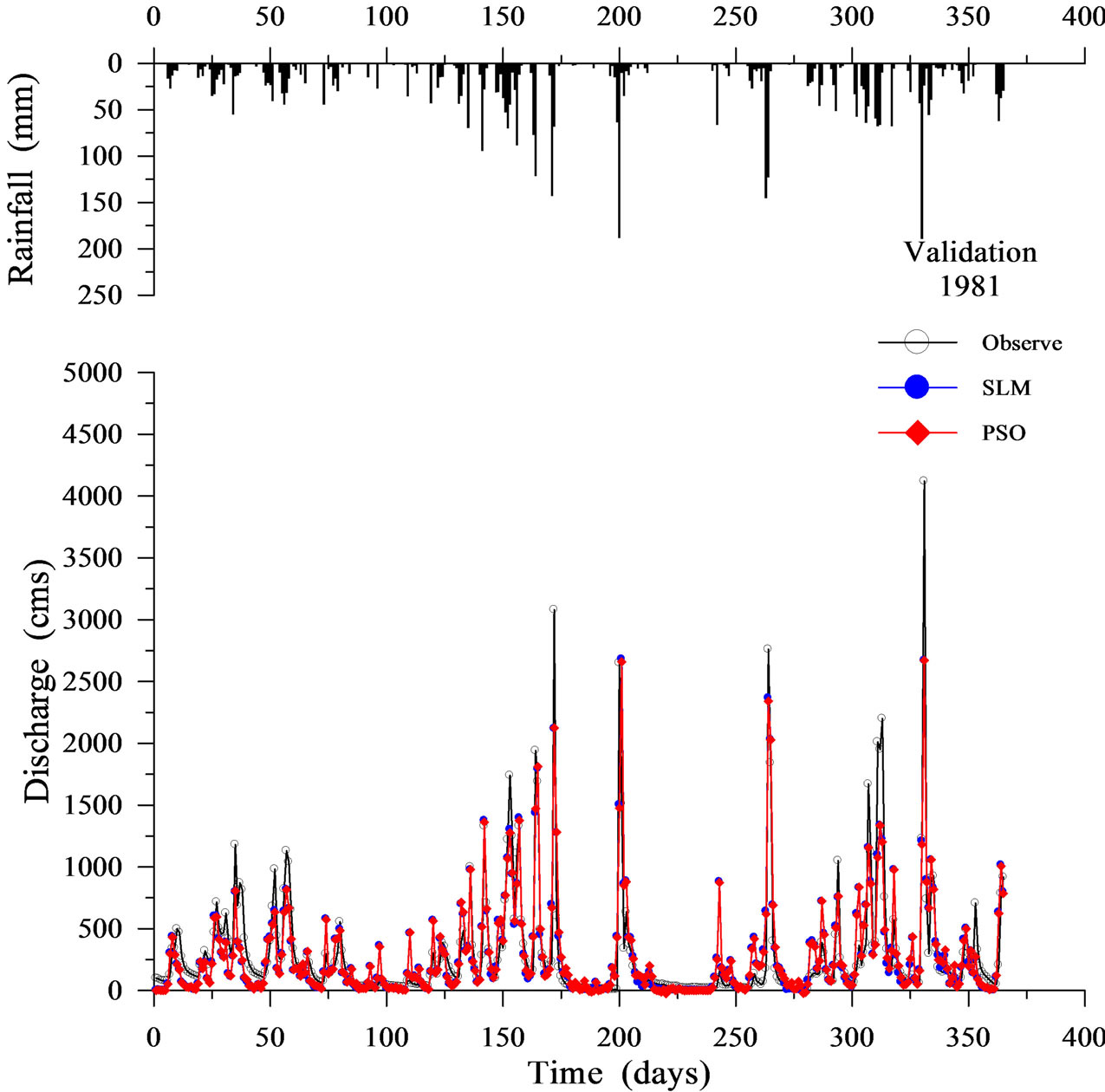
Figure 6. Validation results using SLM and PSO (1981).
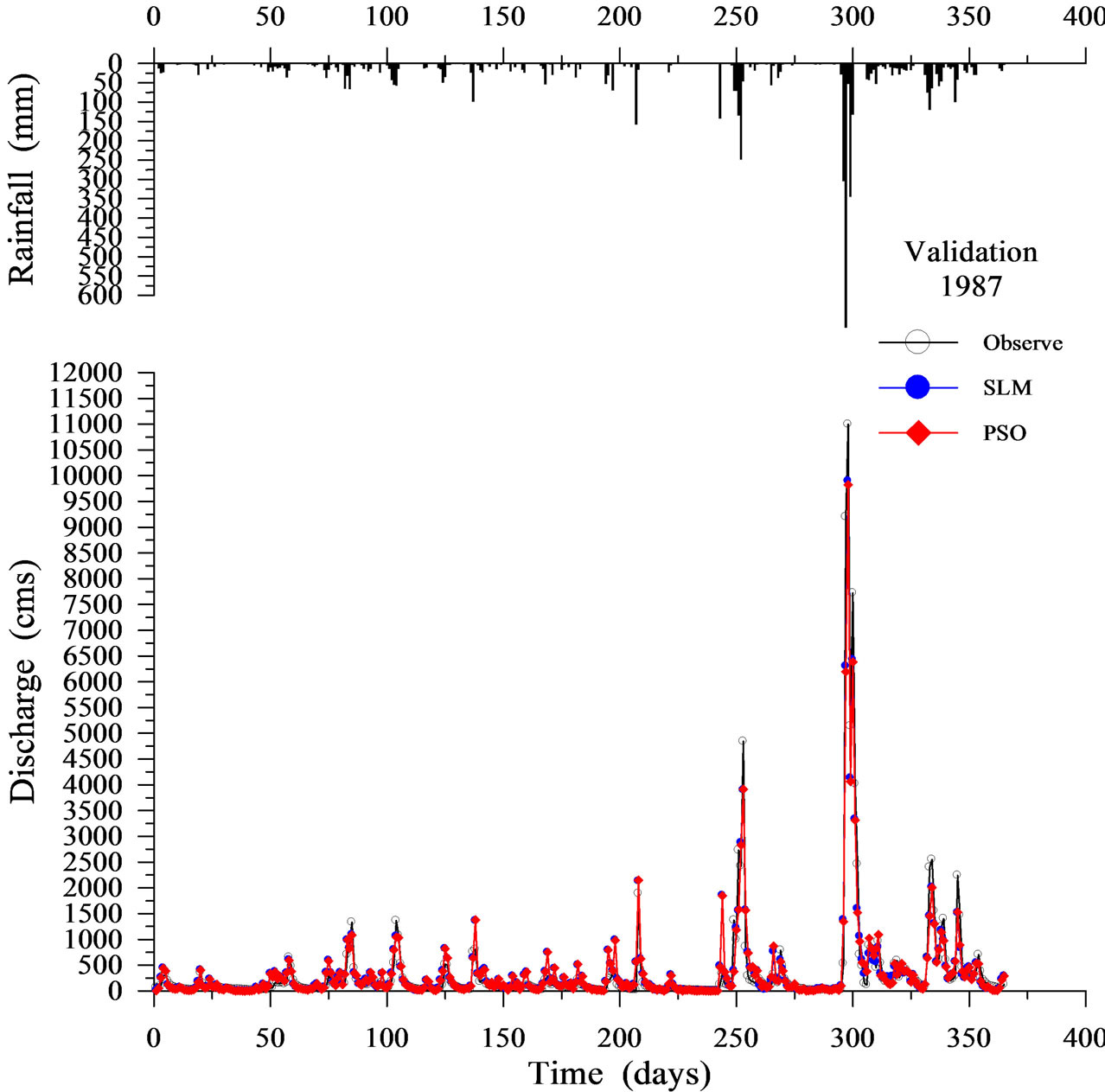
Figure 7. Validation results using SLM and PSO (1987).
Figure 8. Validation results using SLM and PSO (1988).
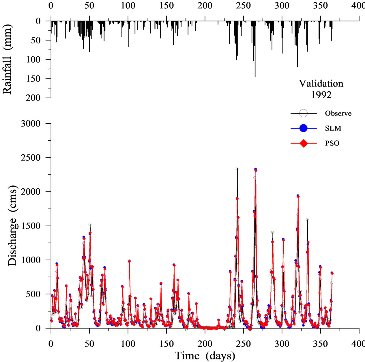
Figure 9. Validation results using SLM and PSO (1992).
tions of all the particles within each generation, play important roles in PSO. In this study, inertia weight coefficient w, and acceleration coefficients c1 and c2 are typically set to 0.5, 2.0 and 2.0, respectively. Much attention should be focused on how to determine their values. In practice, different improved method may be tried in the future regarding the main search procedure of the originnal PSO which is robust.
7. Acknowledgements
The author would like to thank the National Science Council, Taiwan for financially supporting this research under Contract No. NSC 100-2221-E-451-010.
REFERENCES
- C. T. Cheng, C. P. Ou and K. W. Chau, “Combining a Fuzzy Optimal Model with a Genetic Algorithm to Solve Multiobjective Rainfall-Runoff Model Calibration,” Journal of Hydrology, Vol. 268, No. 1-4, 2002, pp. 72-86. doi:10.1016/S0022-1694(02)00122-1
- K. W. Chau, C. L. Wu and Y. S. Li, “Comparison of Several Flood Forecasting Models in Yangtze River,” Journal of Hydrologic Engineering, Vol. 10, No. 6, 2005, pp. 485-491. doi:10.1061/(ASCE)1084-0699(2005)10:6(485)
- J. Y. Lin, C. T. Cheng and K. W. Chau, “Using Support Vector Machines for Long-Term Discharge Prediction,” Hydrological Sciences Journal, Vol. 51, No. 4, 2006, pp. 599-612. doi:10.1623/hysj.51.4.599
- C. T. Cheng, W. C. Wang, D. M. Xu and K. W. Chau, “Optimizing Hydropower Reservoir Operation Using Hybrid Genetic Algorithm and Chaos,” Water Resources Management, Vol. 22, No. 7, 2008, pp. 895-909. doi:10.1007/s11269-007-9200-1
- W. C. Wang, K. W. Chau, C. T. Cheng and L. Qiu, “A Comparison of Performance of Several Artificial Intelligence Methods for Forecasting Monthly Discharge Time Series,” Journal of Hydrology, Vol. 374, No. 3-4, 2009, pp. 294-306. doi:10.1016/j.jhydrol.2009.06.019
- C. L. Wu, K. W. Chau and Y. S. Li, “Predicting Monthly Streamflow Using Data-Driven Models Coupled with Data-Preprocessing Techniques,” Water Resources Research, 45, W08432, 2009, 23 Pages. doi:10.1029/2007WR006737
- F. Wang, K. Xing and X. Xu, “A System Identification Method Using Particle Swarm Optimization,” Journal of Xi’an Jiaotong University, Vol. 43, No. 2, 2009, pp. 116- 120 (in Chinese).
- J. Kennedy and R. C. Eberhart, “Particle Swarm Optimization,” Proceedings of IEEE International Conference on Neural Networks, Perth, Vol. 4, 1995, pp. 1942-1948. doi:10.1109/ICNN.1995.488968
- K. W. Chau, “Particle Swarm Optimization Training Algorithm for ANNs in Stage Prediction of Shing Mun River,” Journal of Hydrology, Vol. 329, No. 3-4, 2006, pp. 363-367. doi:10.1016/j.jhydrol.2006.02.025
- M. K. Gill, Y. H. Kaheil, A. Khalil, M. McKee and L. Bastidas, “Multiobjective Particle Swarm Optimization for Parameter Estimation in Hydrology,” Water Resources Research, Vol. 42, W07417, 2006, 14 Pages. doi:10.1029/2005WR004528
- K. W. Chau, “A Split-Step Particle Swarm Optimization Algorithm in River Stage Forecasting,” Journal of Hydrology, Vol. 346, No. 3-4, 2007, pp. 131-135.
- Y. Luo and X. G. Yuan, “Global Optimization for the Synthesis of Integrated Water Systems with Particle Swarm Optimization Algorithm,” Chinese Journal of Chemical Engineering, Vol. 16, No. 1, 2008, pp. 11-15. doi:10.1016/S1004-9541(08)60027-0
- X. S. Zhang, R. Srinivasan, K. G. Zhao and M. V. Liew, “Evaluation of Global Optimization Algorithms for Parameter Calibration of a Computationally Intensive Hydrologic Model,” Hydrological Processes, Vol. 23, No. 3, 2008, pp. 430-441. doi:10.1002/hyp.7152
- W. C. Wang, X. T. Nie and L. Qiu, “Support Vector Machine with Particle Swarm Optimization for Reservoir Annual Inflow Forecasting,” Proceedings of International Conference on Artificial Intelligence and Computation Intelligence (AICI), Sanya, 2010, pp. 184-188. doi:10.1109/AICI.2010.45
- S. Gaur, B. R. Chahar and D. Graillot, “Analytic Elements Method and Particle Swarm Optimization Based Simulation—Optimization Model for Groundwater Management,” Journal of Hydrology, Vol. 402, No. 3-4, 2011, pp. 217-227. doi:10.1016/j.jhydrol.2011.03.016
- Y. X. Wei and L. X. Wang, “Engineering Hydrology,” Water Conservancy and Electricity Press, Beijing, 2005 (in Chinese).
- Y. C. Liang, C. G. Wu, X. H. Shi and H. C. Ge, “Swarm Intelligent Optimization Algorithm—Theory and Application,” Science Press, Beijing, 2009 (in Chinese).
- H. C. Kuo, J. R. Chang and C. H. Liu, “Particle Swarm Optimization for Global Optimization Problems,” Journal of Marine Science and Technology, Vol. 14, No. 3, 2006, pp. 170-181.
- A. Lattermann, “System-Theoretical Modelling in Surface Water Hydrology,” Springer-Verlag, Germany, 1991. doi:10.1007/978-3-642-83819-4