Journal of Water Resource and Protection
Vol. 1 No. 6 (2009) , Article ID: 1071 , 9 pages DOI:10.4236/jwarp.2009.16047
A Diffusion Wave Based Integrated FEM-GIS Model for Runoff Simulation of Small Watersheds
1NIT Warangal, Andhra Pradesh, India
2Department of Civil Engineering, Indian Institute of Technology (IIT) Bombay, Mumbai, India
E-mail: eldho@civil.iitb.ac.in
Received June 20, 2009; revised July 16, 2009; accepted July 24, 2009
Keywords: Diffusion Wave Model, GIS, Interception, Interflow, Philip Infiltration Model, Runoff Simulation
ABSTRACT
In this paper, an integrated model based on Finite Element Method (FEM) and Geographical Information Systems (GIS) has been presented for the runoff simulation of small watersheds. Interception is estimated by an exponential model based on Leaf Area Index (LAI). Philip two term model has been used for the estimation of infiltration in the watershed. For runoff estimation, diffusion wave equations solved by FEM are used. Interflow has been simulated using FEM based model. The developed integrated model has been applied to Peacheater Creek watershed in USA. Sensitivity analysis of the model has been carried out for various parameters. From the results, it is seen that the model is able to simulate the hydrographs with reasonable accuracy. The presented model is useful for runoff estimation in small watersheds.
1. Introduction
Watershed is the fundamental geographical unit for the planning and management of water resources. Various hydrological processes occurring in the watershed are very complex in nature. A careful representation of the hydrological processes is necessary for the hydrologic modeling as it promises better estimates of hydrologic variables for management decisions [1]. Recent advancements in computing and database management technologies offer better physically based hydrological modeling which in turn provide better estimates of hydrologic variables such as infiltration, runoff etc.
Usually interception can be deducted as some percentage of rainfall. If required data is available for estimation of interception, it is better to incorporate it in the rainfall-runoff model. Aston [2] developed an exponential model for calculation of interception loss based on Leaf Area Index (LAI). Jetten [3] has used LAI and cover fraction based interception method in LISEM (LImburg Sediment Erosion Model). Kang et al. [4] observed good agreement between the measured interception and interception obtained from linear regression model based on plant height and LAI.
Infiltration is an important hydrologic process, which must be carefully considered in the hydrologic models. Philip model is one of the commonly used approximate infiltration model. Luce and Cundy [5] used Philip infiltration model to calculate rainfall excess in their overland flow model. Jain et al. [6] used the Philip two term infiltration model, to compute the infiltration in their model.
In steep humid catchments, interflow (through flow) is more likely to be the main form of drainage. Interflow travels laterally through the upper soil layers until it reaches a conveyance system. Jayawardena and White [7, 8] developed a finite element model suitable for catchments where through flow is dominant and applied to two experimental catchments. Sunada and Hong [9] presented a numerical runoff model describing interflow and overland flow on hill slopes.
St. Venant equations of continuity and momentum are the basic equations to simulate runoff routing in a watershed. A complete solution of St. Venant equations may not be worthy at all times, in view of the large computational efforts. The approximations of St. Venant equations like diffusion wave equations or kinematic wave equations may give most appropriate results with reasonable computational efforts. Morris and Woolhiser [10] showed that diffusion wave equations are adequate for highly sub-critical flow and where the downstream boundary conditions are important consideration. Hromadka II and Yen [11] developed a finite difference based diffusion hydrodynamic model and applied it to different civil engineering drainage problems. Hromadka and DeVries [12] and Ponce [13] in their papers have discussed the limitations of kinematic wave modeling and advantages of diffusion wave modeling over kinematic wave modeling.
The Finite Element Method (FEM) is an efficient way to transform partial differential equations in space and time into ordinary differential equations in time. Finite difference schemes may then be used to solve for the time dependent solution of the system [14]. Blandford and Ormsbee [15] used diffusion wave equations to develop a finite element model for dendritic channel network with trapezoidal and rectangular channel geometries.
The physical parameters, which influence runoff routing, such as slope and Manning’s roughness vary spatially over the watershed. Spatial variation of these properties can be better incorporated into the model by using Geographical Information Systems (GIS). Sui and Maggio [16], Garbrecht et al. [17] and Vieux [14] discussed the use of GIS in watershed modeling. Jaber and Mohtar [18] developed a GIS interface for the overland flow model by using the ArcView 3.2. In this paper an integrated hydrologic model based on FEM and GIS is presented for the runoff simulation and to analyze its application to a small watershed.
2. Model Formulation
In this paper, finite element based rainfall-runoff model using GIS is described for the simulation of event based surface runoff. Diffusion wave equations are used in the model development. Galerkin FEM technique has been used in the solution of the governing equations. Interception has been estimated by an exponential model based on Leaf Area Index (LAI). Philip two term infiltration model has been used for the estimation of infiltration. Interflow has been estimated using FEM based model. Finite element grid has been prepared for the watershed by using GIS. Spatially distributed information for model inputs such as slope and Manning’s roughness are provided for each node of FEM grid using GIS.
2.1. Interception Model
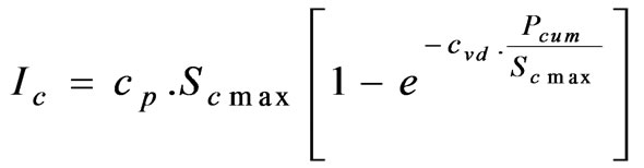
Interception is estimated based on the equations used in the LISEM model [3]. In this model, canopy of crops and vegetation is regarded as simple storage. The cumulative interception during an event is given as [2]:
 (1)
(1)
where Ic is the cumulative interception, cpis the fraction of vegetation cover, cvd is the correction factor for vegetation density and is given as cvd=0.046×LAI, Pcum is the cumulative rainfall, Scmax is the canopy storage capacity and LAI is the Leaf Area Index. Canopy storage capacity Scmax is calculated by equation developed by Von Hoyningen-Huene [3] as follows:
 (2)
(2)
The interception loss ( ) for every time step is calculated as follows:
 (3)
(3)
where t is the time and Δt the time step. Interception rate from the interception loss has been calculated and is deducted from rainfall intensity to get the effective rainfall intensity which is used to calculate infiltration and subsequent runoff.
2.2. Philip Two-Term Infiltration Model
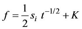
The Philip two term infiltration model is used for computing the infiltration. The rate of infiltration given by Philip in 1957 [19] is as follows:
 (4)
(4)
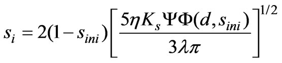
where ƒ is the infiltration rate as a function of time, Si is the infiltration sorptivity and K is the hydraulic conductivity which is considered equal to the saturated hydraulic conductivity (Ks). Infiltration sorptivity si [20] can be expressed as follows:
 (5)
(5)
where sini is the initial (uniform) soil saturation degree in the surface boundary layer, is the saturated matrix potential of the soil,
  is the dimensionless surface sorption diffusivity of the soil, η is the effective porosity of the soil, λ is pore size distribution index and d is the diffusivity index.
Here ,
, and d have been calculated based on the expressions given by Jain et al. [6]. Infiltration rate (ƒ) has been estimated based on the equations given by Chow et al. [19]. The soil parameter Si can be calculated using soil dependent parameters of η, λ, Ks and sini. The standard values of η, λ, Ks are available in literature for various soil types. These are used as a first approximation in the model and optimum values can be estimated by calibration. The initial soil saturation degree sini.has been assumed randomly for each rainfall event and optimal value can be estimated by calibration.
2.3. Governing Equations for Surface Runoff
In a watershed, surface runoff can be divided into overland flow and channel flow. Overland and channel flow are formulated based on diffusion wave equations to route the runoff to outlet of the watershed.
2.3.1. One Dimensional Diffusion Wave Equation for Overland Flow
The continuity and momentum equations for diffusion wave for overland flow are given as [21]:
 (6)
(6)
 (7)
(7)
where q is the flow per unit width, h is the depth of flow; re is the excess rainfall intensity after interception and infiltrations loss, x is the variable representing space,  is the variable representing time, So is the slope of overland flow plane and Sƒ is the friction slope of flow plane. The flow per unit width is given as q=αhβ. α andβcan be derived by using Manning’s equation and are given as
  and
and , where
  is the overland flow Manning’s roughness coefficient.
The above governing equations are solved using initial and boundary conditions. Initial condition is of no flow condition and it is given as at time t=0; h=0 and q=0 at all nodal points. Upstream boundary condition is assumed as zero inflow and it is given as h=0 q=0 at all times t. Downstream boundary condition is of zero depth gradient [22] and it is expressed as (әh/әx)=0 at all times t. This condition can also be written with the end node M as hM=hM-1.
2.3.2. One Dimensional Diffusion Wave Equation for Channel Flow
Diffusion wave equation for channel flow consists of continuity and momentum equations as:
 (8)
(8)
 (9)
(9)
where  is the discharge in the channel,
  is the area of flow in the channel,
  is the bed slope of channel and
  is the friction slope of channel.
  in Equation (8) can be represented by the uniform flow equation such as Manning’s equation and is given as follows:
 (10)
(10)
where R is the hydraulic radius (A/P),P is the wetted perimeter and nc is the channel flow Manning’s roughness coefficient. By substituting for R in Equation (10) gives:
 (11)
(11)
Initial condition is given as: at time  = 0;
= 0; 
 and
and . Upstream boundary condition is of zero inflow and it is given as
  and
and . Downstream boundary condition is of zero depth gradient and it is similar to overland flow.
2.3.3. Finite Element Formulation for Overland Flow
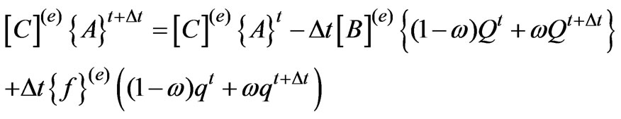
Here, one dimensional line elements are used for spatial discretization. Applying the Galerkin finite element formulation [23] to Equation (6) gives:
 (12)
(12)
where ,
, and
and  are elemental matrices. The super scripts
  and
and  indicate the variables at the previous time step and current time step.
  is the factor that determines the type of finite difference scheme involved. Here Crank-Nicolson scheme with
  is used. Equation (12) is applied to all elements in the domain and assembled to form a system of equations. The system of equations is solved by Cholesky scheme after applying the boundary conditions for the unknown values of
 . The solution of
  requires iteration due to non-linearity of the Equation (12). Iteration is continued until the convergence is reached to a specified tolerance value (
 ). After convergence on
 , the time step is incremented and the solution proceeds in the same manner by updating the time matrices and evaluating the new
  values. During calculation of friction slope, the following formulation has to be applied in explicit finite difference form for the Equation (7) [6].
 (13)
(13)
where  and
and  represent successive nodes in flow direction and L is the length of element.
2.3.4. Finite Element Formulation for Channel Flow
Here, continuity Equation (8) is approximated using Galerkin FEM. The final form of the FEM equation which will be used in the channel flow model is as follows.
 (14)
(14)
As in the case of overland flow, Equation (14) is applied to all elements and assembled to form a system of equations, which are solved after application of boundary conditions.
2.4. Interflow Model
Interflow model has been formulated based on the through flow equations given by Jayawardena and White [7]. The continuity equation for the interflow is as follows:
 (15)
(15)
where qi is the interflow, hi is the saturated layer thickness in which interflow passes, η is the porosity of the interflow zone same as in the infiltration model and Ii is the lateral recharge rate due to infiltration per unit area. The interflow qi can be expressed by Darcy’s law for flow in porous media, in a direction parallel to the overland flow plane slope (S0) and is given as qi=K S0 hi Here K is the hydraulic conductivity of the interflow zone, same as in infiltration model. Substituting qi in Equation (15) gives the interflow as:
2.4.1. Finite Element Formulation
By applying Galerkin finite element formulation to Equation (15), the final form of equation is as follows:
 (16)
(16)
As in the case of overland flow, Equation (16) is applied to all elements of overland flow plane and assembled to form a system of equations and solved.
3. Model Development and Evaluation
Based on the above formulation, computer models were developed for interception model, Philip infiltration model, surface runoff routing model based on diffusion wave formulation and interflow model, using C programming language. Further these models are integrated together for the prediction of runoff at any location for the given rainfall conditions. Infiltration from the Philip model is the input to the interflow model assuming that some part of infiltration flows towards the stream through a saturated zone and contributes to the runoff. Finite element mesh and input data required for the integrated model has been prepared using the GIS.
3.1. Model Evaluation
The developed integrated model has been evaluated on the Peacheater Creek watershed in USA. The data required for Peacheater Creek watershed is available in Distributed Model Inter comparison Project (DMIP) website
(http:// www.nws.noaa.gov/oh/hrl/dmip/ index. html). Some data like watershed boundary, stream flow data and gauging
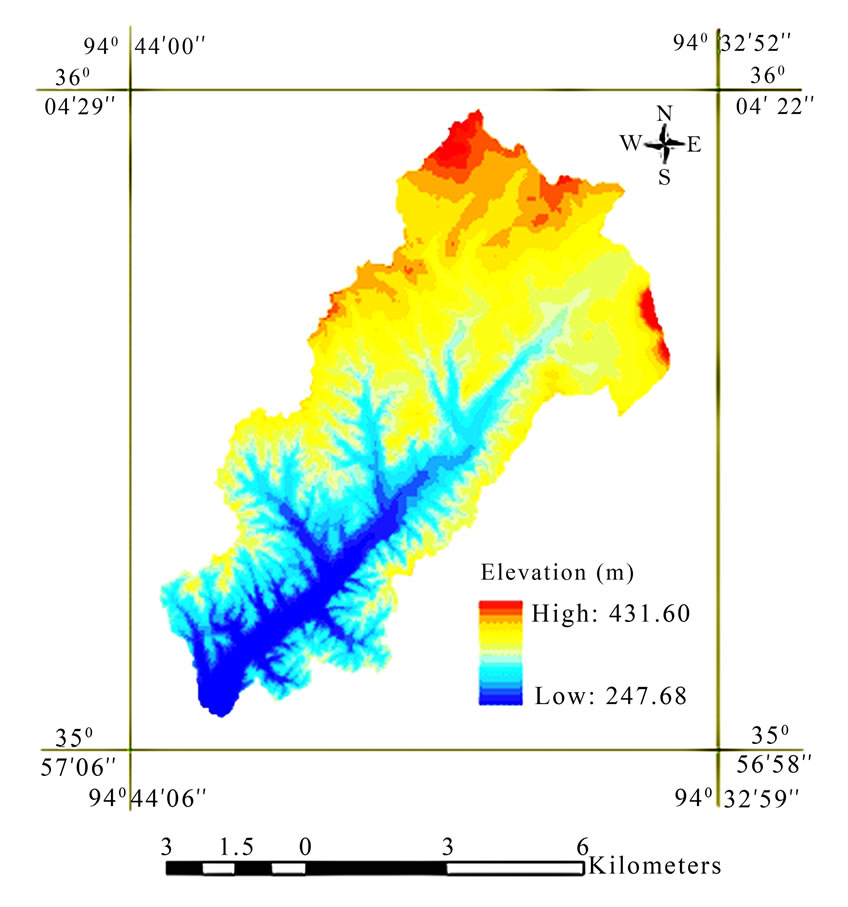
Figure 1. Digital Elevation Model of Peacheater Creek watershed.
station information are obtained through personal communication (Michael B. Smith and Seann M. Reed, DMIP, National Weather Service Office of Hydrologic Development, USA, 2005).
3.2. Study Area and Preparation of Database
The Peacheater creek watershed is one of the study watersheds of DMIP. It has an area of 63.58 km2. It is a gauged sub-watershed of Baron Fork catchment, Oklahoma, USA. Gauging station for this watershed is located at Christie, Oklahoma. The watershed consists primarily of silt loam soils with forested (42%), grassy (57%) and urban (1%) areas [24]. ASCII files of DEM (1 arc-second), soil and land use map of the Baron Fork basin with 30 m grid resolution were converted into map format with appropriate projection information. Required DEM, soil and land use maps for Peacheater creek watershed are clipped, based on the boundary of the watershed. DEM of the watershed is shown in Figure 1. Drainage map of the watershed is generated based on DEM using Hydrology tools of ArcMap. Percentage slope map is prepared from DEM by using the slope option of Spatial Analyst in ArcMap. The percentage slope is then converted in to slope values by Raster Calculator option in GIS. Hourly rainfall data in binary format were obtained from DMIP website (Stage 3 Next-Generation Weather Radar (NEXRAD) observations at 4x4 km resolution). Based on the procedure explained in the DMIP website, the hourly rainfall maps are prepared and clipped for the watershed.
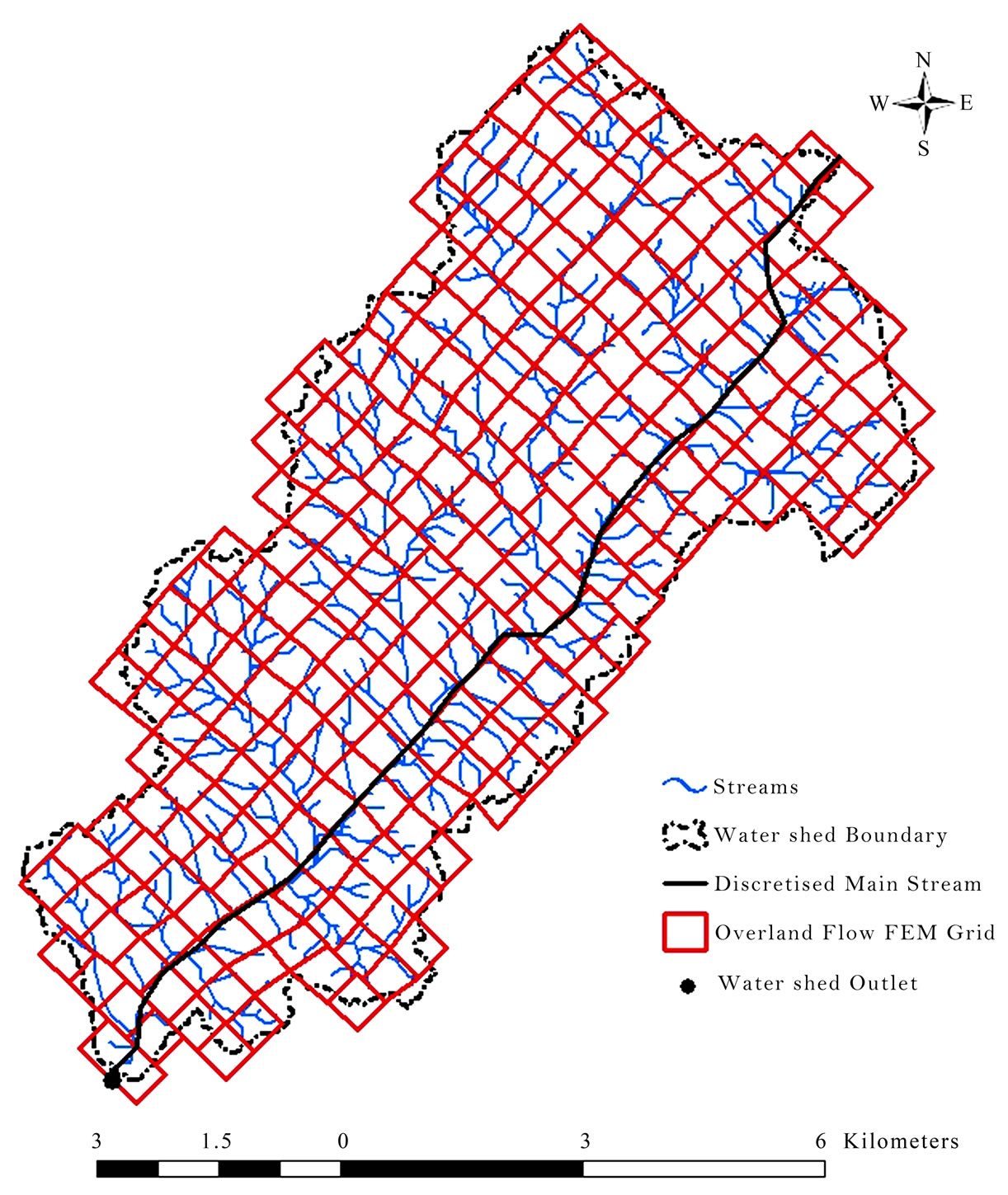
Figure 2. Peacheater creek watershed with FEM grid.

Table 1. Calibrated parameters for rainfall events.
FEM grid map of the watershed is prepared with overland flow strips with element size of 500x500m., as shown in Figure 2. The grid map has been overlaid on slope map. By using the Zonal Statistics option in the Spatial Analyst module of ArcMap, the mean value of slope has been calculated for each element of the grid. The attribute table of the grid containing the element number and mean value of slope has been exported as database file. The present model needs input data of slope at the nodal level. It is obtained by taking average of adjacent element values.
3.3. Model Simulation
The developed model has been applied to simulate the runoff in Peacheater Creek watershed for six rainfall events. A constant channel width of 45 m, slope 0.006, time step 30 s, η of 0.416 and λ of 0.28 have been used in the simulation of rainfall events. In view of the non availability of data for the interception model, LAI of 1.5 and cp of 0.5 have been assumed.
The model has been calibrated for four rainfall events
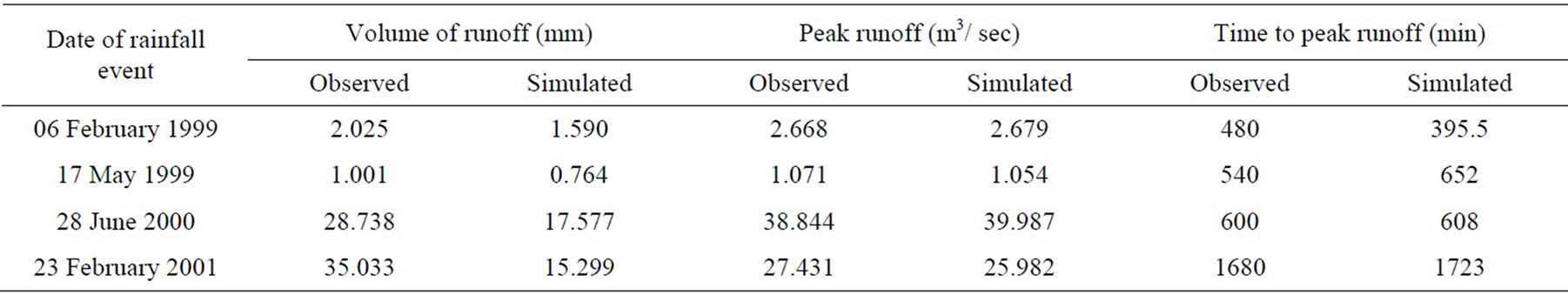
Table 2. Model results for the calibration storms.
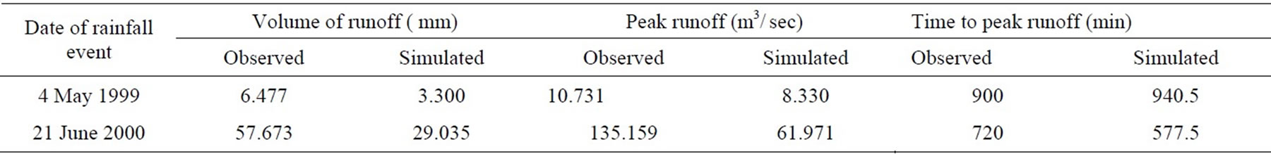
Table 3. Model results for the validation storms.
 (a)
(a)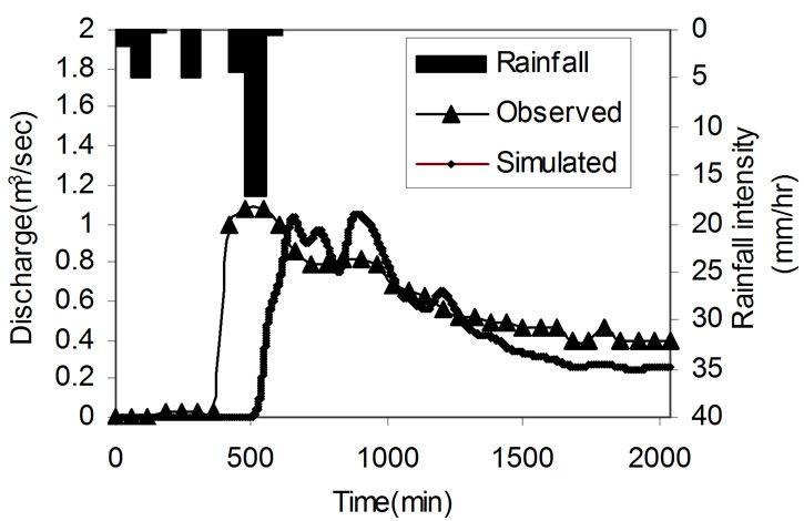 (b)
(b)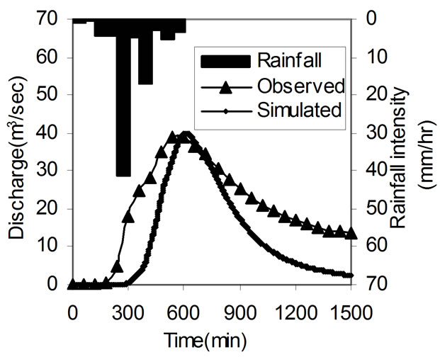 (c)
(c) (d)
(d)
Figure 3. Observed and simulated hydrographs for calibration events; (a) 06 February 1999; (b) 17 May 1999; (c) 28 June 2000; (d) 23 February 2001.
of Peacheater Creek watershed. Validation of model has been carried out with two rainfall events. Calibration has been performed by altering the values of Ks and Sini by trial and error based on the best visual fit of the hydrographs. The parameters no and nc have been calibrated in the absence of data. Calibrated parameters for Peacheater Creek watershed are given in Table 1. The model fit was checked based on the difference between observed and computed volume of runoff, peak runoff and time to peak. Validation of two rainfall events of Peacheater watershed is carried out by taking average parameters of four calibrated rainfall events.
4. Results and Discussions
The observed and simulated hydrographs for the four calibrated rainfall events of Peacheater Creek watershed are shown Figure 3. Table 2 shows the observed and simulated values of volume of runoff, peak runoff and time to peak runoff for the four calibrated events. From the simulation results, it is seen that volume of flow has been simulated within variation of  56% and peak flow within variation of
  6% and time to peak within a variation of
  21%.
21%.
The observed and simulated hydrographs for the two validated events of Peacheater Creek watershed are shown in Figure 4. Table 3 shows the observed and simulated values of volume of runoff, peak runoff and time to peak runoff for the two validated events. From the validation of simulation results, it is seen that volume of flow has been simulated within a variation of  50% and peak flow within a variation of
  54% and time to peak within a variation of
  20%.
20%.
Topographic complexity in the Peacheater Creek controls the catchment response to rainfall via interactions between the active shallow aquifer, stream network and land surface [24]. Even though the present model has been simulating interflow, it is unable to simulate perched return flow and ground water exfiltration which are important hydrological processes of this watershed. In addition, the channel slope and width values are assumed to be constant throughout the length of the channel, because of lack of data, and weighted average rainfall for the whole watershed has been used in the model. These factors might have contributed to the discrepancy between the observed and simulated flow.
Also a sensitivity analysis of the model has been carried out by altering the parameters of Ks, Sini, no and nc by  10%. Effect of change in calibrated parameters on computed values of volume of runoff, peak runoff and time to peak runoff are shown for a rainfall event in Figure 5. From the results, it is observed that the values of computed volume of runoff and peak runoff are most sensitive to Ks followed by no, nc and Sini. The value of computed time to peak runoff is most sensitive to nc followed by no, Ks and Sini The change of
  10% in the parameter Ks caused a variation of 12% in the volume of runoff and peak runoff and 0.5% variation in the time to peak. The change of
  10% in the parameter no caused a variation of 6% in the volume of runoff and peak runoff and 1.7% variation in the time to peak. The change of
  10% in the parameter nc caused a variation of 0.9% in the volume of runoff and 4.4% in the peak runoff and 2.4% variation in the time to peak. It indicates that volume of runoff is more sensitive to the infiltration parameters than flow resistance parameters and time to peak is more sensitive to the flow resistance parameters than infiltration parameters. It is also seen that peak runoff is sensitive to both infiltration and flow resistance parameters. The change of
  10% in the parameter Sini caused a variation of 1% in the volume of runoff and peak runoff and 0.1% variation in the time to peak. It indicates that volume of runoff, peak runoff and time to peak runoff are least sensitive to Sini. This may be true since most of the rainfall events simulated are long duration events where initial saturation conditions may not have much influence on the flow parameters. However, it is observed from the sensitivity analysis that all the parameters considered are important in the simulation of runoff and accuracy of these parameters control the accuracy of the simulation results.
5. Concluding Remarks
An integrated FEM and GIS based rainfall runoff model using diffusion wave equation is presented here. Interception has been calculated by an empirical model based on Leaf Area Index (LAI). Philip two-term infiltration model is used for estimation of infiltration. Interflow model has been developed using FEM. The developed model has been calibrated and validated on Peacheater Creek watershed in USA.
The developed model has fairly simulated the hydrographs at the outlet of watershed. From the simulation results of watershed, it is seen that volume of runoff has been simulated within variation of  56%, peak runoff within variation of
  6% and time to peak runoff within variation of
  21% for calibrated rainfall events.
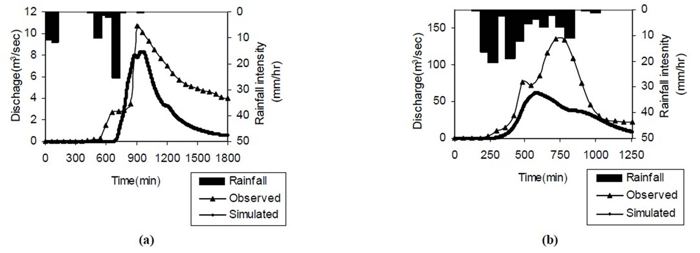
Figure 4. Observed and simulated hydrographs for validation events; (a) 4 May1999; (b) 21 June 2000.
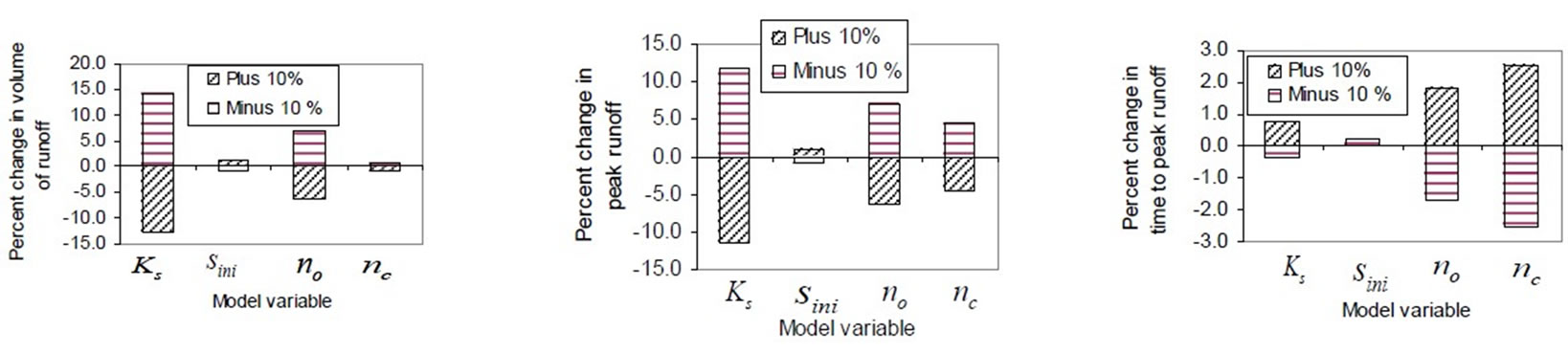
Figure 5. Effect of change in calibrated model parameters on computed values of volume of runoff, peak runoff and time to peak runoff (28 June 2000).
Model performed well on some of the validation rainfall events. This may be primarily due to differences in characteristics between the calibration storms and the validation storms. Large variation in simulated volume of runoff for some of the rainfall events may be because of simulated interflow not representing the perched return flow and ground water exfiltration which are important hydrological processes of this watershed. Further, sensitivity analysis for various parameters has been carried out. From the sensitivity analysis results, it is seen that volume of runoff is more sensitive to the infiltration parameters than flow resistance parameters and time to peak is more sensitive to the flow resistance parameters than infiltration parameters. It is also observed that all the infiltration and flow resistance parameters considered in the model are important in the simulation of runoff.
The model in its present form is not suitable during hiatus and prolonged interstorm periods because it doesn’t account for moisture balance and evapo-transpiration losses. In the present study calibrated values of infiltration and flow resistance parameters based on the observed hydrographs have been used in the simulation. The present study, demonstrated the application of GIS in simulation of runoff by integration of FEM based surface runoff and interflow models and conceptually established interception and infiltration models. The model presented here can be applied to agricultural and forested watersheds since this model will take care of interflow and interception. The model can be applied to small to medium watersheds for the event based runoff simulation. Due to lack of availability of suitable data, the model applicability for larger watersheds could not be carried out.
6. Acknowledgements
Authors are thankful to the ISRO-IITB cell for the financial assistance to carryout this work through project No. 03IS007. Authors are also thankful to Michael B. Smith and Seann M. Reed, DMIP, National Weather Service, Office of Hydrologic Development, Sliver Spring, USA for providing the database of Peacheater Creek watershed, Oklahoma, USA.
REFERENCES
- L. D. James and S. J. Burges, “Selection, calibration, and testing of hydrologic models,” Hydrologic Modeling of Small Watersheds (C. T. Haan, H. P. Johnson and D. L. Brakensiek (Eds.)), Monograph, ASAE, Michigan, USA, No. 5, pp. 437–472, 1982.
- A. R. Aston, “Rainfall interception by eight small trees,” Journal of Hydrology, Vol. 42, pp. 383–396, 1979.
- V. Jetten, “LISEM Limburg Soil Erosion Model,” Windows version 2.x, USER MANUAL, Utrecht University, Netherlands, pp. 7–7, 2002. See http://www.geog.uu.nl/lisem for further details, Accessed 26/08/2005.
- Y. Kang, Q. G. Wang, and H. J. Liu, “Winter wheat canopy interception and its influence factors under sprinkler irrigation,” Agricultural Water Management, Vol. 74, pp. 189‑199, 2005.
- C. H. Luce and T. W. Cundy, “Modification of the kinematic wave-Philip infiltration overland flow model,” Water Resources Research, Vol. 28, No. 4, pp. 1179– 1186, 1992.
- M. K. Jain, U. C. Kothyari, and K. G. R. Raju, “A GIS based distributed rainfall-runoff model,” Journal of Hydrology, Vol. 299, pp. 107–135, 2004.
- A. W. Jayawardena and J. K. White, “A finite element distributed catchment model, I. Analytical basis,” Journal of Hydrology, Vol. 34, pp. 269–286, 1977.
- A. W. Jayawardena and J. K. White, “A finite element distributed catchment model, II. Application to the real catchments,” Journal of Hydrology, Vol. 42, pp. 231–249, 1979.
- K. Sunada and T. F. Hong, “Effects of slope conditions on direct runoff characteristics by the interflow and overland flow model,” Journal of Hydrology, Vol. 102, pp. 323–334, 1988.
- E. M. Morris and D. A. Woolhiser, “Unsteady onedimensional flow over a plane: Partial equilibrium and recession hydrographs,” Water Resources Research, Vol. 16, No. 2, pp. 355–360, 1980.
- T. V. Hromadka II and C. C. Yen, “A diffusion hydrodynamic model (DHM),’’ Advances in Water Resources, Vol. 9, No. 9, pp. 118–170, 1986.
- T. V. Hromadka II and J. J. Devries, “Kinematic wave routing and computational error,” Journal of Hydraulic Engineering, Vol. 114, No. 2, pp. 207–217, 1988.
- V. M. Ponce, “Kinematic wave modeling: Where do we go from here?” in International Symposium on Hydrology of Mountainous Areas, National Institute of Hydrology, Shimla, India, 1992.
- B. E. Vieux, “Distributed Hydrologic Modeling Using GIS,” Kluwer Academic Publishers, Dordrecht, Netherlands, 2001.
- J. E. Blandford and E. L. Ormsbee, “A diffusion wave finite element model for channel networks,” Journal of Hydrology, Vol. 142, pp. 99–120, 1993.
- D. Z. Sui and R. C. Maggio, “Integrating GIS with hydrological modeling: practices, problems, and prospects,” Computers, Environment and Urban Systems, Vol. 23, No. 1, pp. 33–51, 1999.
- J. Garbrecht, F. L. Ogden, P. A. Debarry, and D. R. Maidment, “GIS and distributed watershed models. I: Data coverages and sources,” Journal of Hydrologic Engineering, Vol. 6, No. 6, pp. 506–514, 2001.
- F. H. Jaber and R. H. Mohtar, “Stability and accuracy of two dimensional kinematic wave overland flow modeling,” Advances in Water Resources, Vol. 26, No. 11, pp. 1189–1198, 2003.
- V. T. Chow, D. R. Maidment, and L. W. Mays, “Applied hydrology,” McGraw-Hill, New York, USA, 1988.
- P. S. Eagleson, “Climate, soil and vegetation 3. A simplified model of soil moisture movement in liquid phase,” Water Resources Research, Vol. 14, No. 5, pp. 722–730, 1978.
- V. P. Singh, “Kinematic wave modeling in water resources.” John Wiley and Sons, New York, USA, 1996.
- E. M. Morris, “The effect of the small slope approximation and lower boundary condition on solutions of Saint-Venant equations,” Journal of Hydrology, Vol. 40, pp. 31–47, 1979.
- J. N. Reddy, “An Introduction to the finite element method,” McGraw Hill, New York, USA, 1993.
- E. R. Vivoni, V. Y. Ivanov, R. L. Bras, and D. Entekhabi, “On the effects of triangulated terrain resolution on distributed hydrologic model response,” Hydrological Processes, Vol. 19, pp. 2101–2122, 2005.