Journal of Software Engineering and Applications
Vol. 5 No. 4 (2012) , Article ID: 18569 , 24 pages DOI:10.4236/jsea.2012.54028
Lyapunov-Based Dynamic Neural Network for Adaptive Control of Complex Systems
![]()
Unité de Recherche LARA Automatique, Ecole Nationale d’Ingénieurs de Tunis (ENIT), Tunis, Tunisia.
Email: zouari.farouk@gmail.com, {kamel.bensaad, mohamed.benrejeb}@enit.rnu.tn
Received December 14th, 2011; revised January 17th, 2012; accepted February 20th, 2012
Keywords: Complex Dynamical Systems; Lyapunov Approach; Recurrent Neural Networks; Adaptive Control
ABSTRACT
In this paper, an adaptive neuro-control structure for complex dynamic system is proposed. A recurrent Neural Network is trained-off-line to learn the inverse dynamics of the system from the observation of the input-output data. The direct adaptive approach is performed after the training process is achieved. A Lyapunov-Base training algorithm is proposed and used to adjust on-line the network weights so that the neural model output follows the desired one. The simulation results obtained verify the effectiveness of the proposed control method.
1. Introduction
For several decades, the problem of adaptive control of complex dynamic systems causes the interest of automation specialists. The use of Proportional-Integral-Derivative (PID) controllers is simple to perform, that give poor performance if there are uncertainties and nonlinearities in the system to be controlled. In several references like [1-3], neural networks are presented as tools to solve control problems due to their ability to model systems without analyzing them theoretically and their possessions a great capacity for generalization, which gives them a good robustness to noise [4].
Several strategies of the neural adaptive control exist which we quote: direct adaptive neural control, indirect adaptive neuronal control, adaptive neural internal model control, adaptive depth control based on feedforward neural networks, robust adaptive neural control, FeedbackLinearization based neural adaptive control, adaptive neural network model based nonlinear predictive control [5-13]. Each strategy has neural adaptive control architecture, the algorithms used during the calculation of the parameters and stability conditions. It has three types of neural adaptive control architectures. The first type of architecture consists of a neural controller and a system to be controlled. The second type of neural architecture includes a controller, a system to be controlled and his neural model. The third type of architecture is composed of a neuronal controller, one or more robustness filter, a system to be controlled and his neural model.
The adjustment of the model parameters and the controller is performed by neural learning algorithms that are based on the choice of the criterion to minimize, a minimization method and the theory of Lyapunov for stability and borniture of all signals existing. Several minimization methods exist which are presented: simple gradient method, gradient method with variable pitch, Newton method and Levenberg-Marquardt method [14].
The contribution of this paper is to propose an adaptive Lyapunov-Based control strategy for complex dynamic system. The control structure takes advantage of Artificial Neural Network (ANN) learning and generalization capabilities to achieve accurate speed tracking and estimation. ANN-Based controllers lack stability proofs in many control structure applications and tuning them in a cascaded control structure is a difficult task to undertake. Therefore, we proposed a Lyapunov stability-Based adaptation technique as an alternative to the conventional gradient-Based and heuristic tuning methods. Thus, the stability of the proposed approach is guaranteed by Lyapunov Stability direct method unlike many computational intelligenceBased controllers.
The different sections of this paper are organized as follows: in Section 2, we present the considered recurrent neural network and the proposed Lyapunov learning algorithm used for updating the weight parameters of the model system.
The proposed adaptive control approach training while a Lyapunov Stability-Based adaptation algorithm is detailed in Section 3. Numerical results are reported and discussed in Section 4, and a conclusion is drawn in Section 5.
2. Neural Network Modeling Approach
Neural network modeling of a system from samples affected by noise usually requires three steps. The first step is the choice of neural network architecture, that is to say, the number of neurons in the input layer which is a function of past values of the input and output, the number of hidden neurons, the number of neurons in the output layer neurons and the organization of them. The work [15,16] show that every continuous function can be approximated by a neural network with three layers, the activation functions of neurons are respectively the sigmoid function for hidden layer neurons and linear function for neurons in the output layer. There are two types of architectures of multilayer neural networks: neural networks, non-curly (static networks) and neural networks curly or recurrent (dynamic networks). Neural networks are non curly most used in the identification and control systems [17]. They may not be powerful enough to model complex dynamic systems with respect to neural networks curly. Different types of recurrent neural networks have been proposed and have been successfully applied in many fields [18-25]. The structure of fully connected recurrent neural networks which was proposed by Williams and Zipser [26], is most often used [27,28] because of its generality. The second step is learning or in other words, estimating the parameters of the network from examples of input-output system identification. The methods of learning are numerous and depend on several factors, including the choice of error function, the initialization of weights, and the selection of the learning algorithm and the stopping criteria of learning. Learning strategies were presented in several research works that we cite [29-31]. The third step is the validation of the neural network obtained using the testing criteria for measuring performance. Most of these tests require a data set that was not used in learning. Such a test set or validation should, if possible, cover the same range of operation given that all learning.
2.1. Architecture of the Recurrent Neural Network
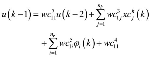
In this work, we consider a recurrent neural network (Figure 1) for identification of complex dynamic systems to a single input and single output. The architecture of these networks is composed of two parts: a linear model the linear behavior of the system and a non-linear approach to nonlinear dynamics.
where:
 is the output of the neural network at time
 ,
,
 and y are respectively the input and output system to identify,
 and
and  are the activation fun-
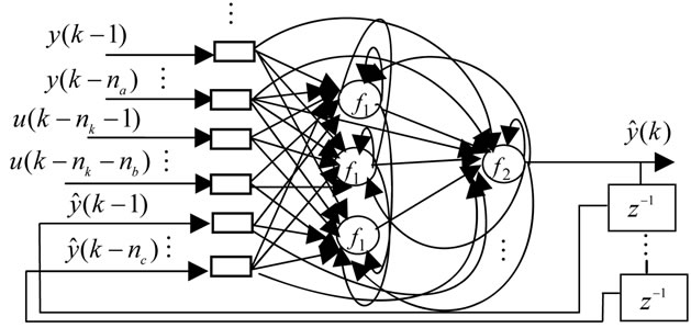
Figure 1. Architecture of the considered neural network.
ctions of neurons,
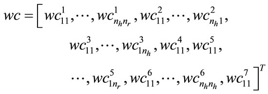
 the number of neurons in the hidden layer respectively of the model and controllerThe coefficients of the vector of parameters of the neural model
 are decomposed into 7 groups, formed respectively by:
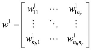 the weights between neurons in the input layer and neurons in the hidden layer,
 the bias of neurons in the hidden layer,
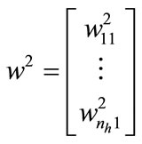
 the weights between neurons in the hidden layer neurons and output layer,
 the bias of neuron in the output layer,
 the weights between neurons of input layer neurons and output layer,
 the weights between neurons
in the hidden layer,
 back weight of neuron in the output layer,
 the outputs of the hidden layer of neural model,
 number of neurons in the input layer.
 (1)
(1)
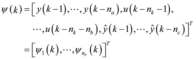
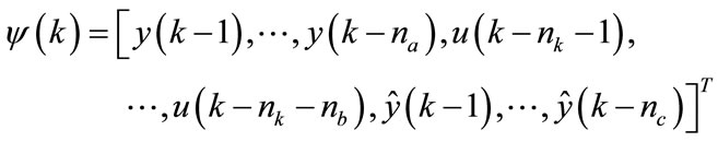
The vector of parameters of the neural model is defined as:
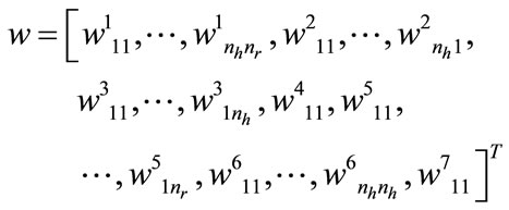 (2)
(2)
The output of neural model  is given by:
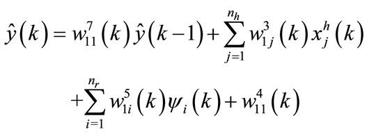 (3)
(3)
such as:
 (4)
(4)
 (5)
(5)
 (6)
(6)
 (7)
(7)
The neural model of the system can be expressed by the following expression:
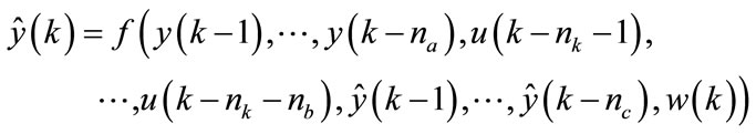 (8)
(8)
2.2. Proposed Lyapunov-Base Learning Algorithms
Several Lyapunov stability-based ANN learning techniques are also proposed to insure the ANNs’ convergence and stability [32,33]. In this section we present three learning procedures of neural network.
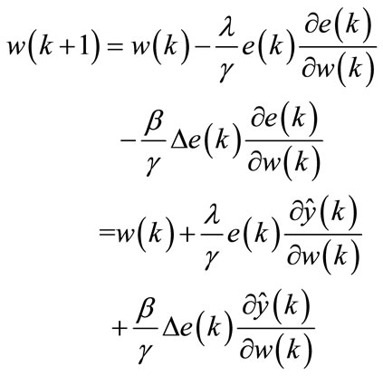
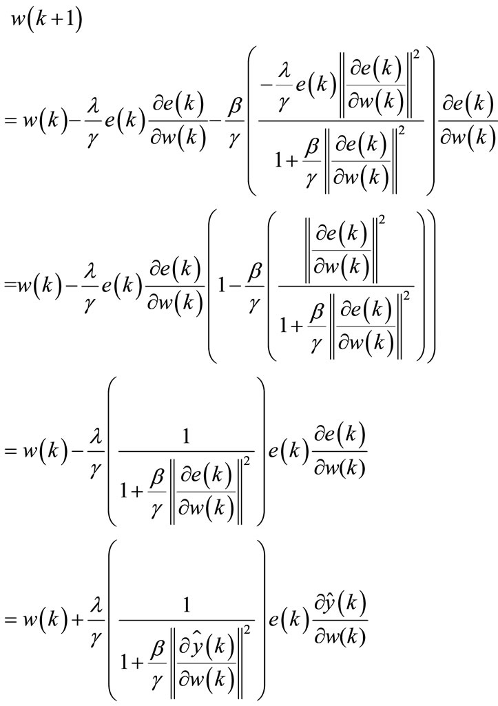
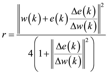
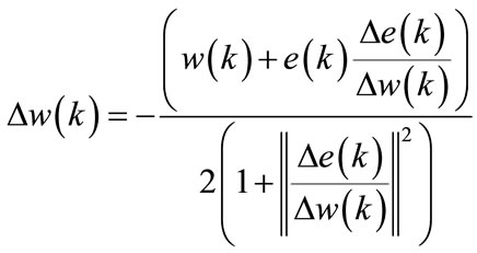
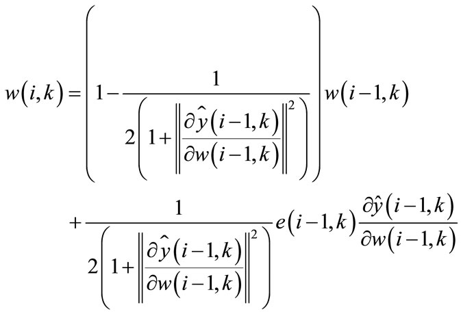
Theorem 1. The learning procedure of a neural network can be given by the following equation:
 (9)
(9)
such as:
 (10)
(10)
 (11)
(11)
 is the Euclidean norm.
wang#title3_4:spProof:
Considering the following quadratic criterion:
 (12)
(12)
 (13)
(13)
 (14)
(14)
The learning procedure is to adjust the coefficients of the neural networks considered by minimizing the criterion  ; it is necessary to solve the equation:
 (15)
(15)
therefore:
 (16)
(16)
According to reference [34], the difference in error due to learning can be calculated by:
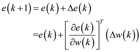 (17)
(17)
The term  is then written as follows:
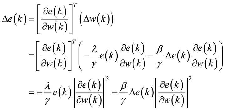 (18)
(18)
Therefore:
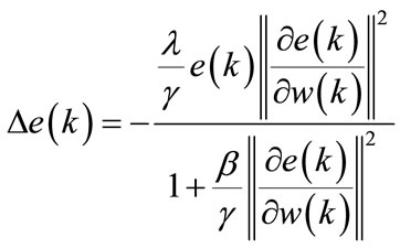 (19)
(19)
According to Equations (16) and (19), we can write:
 (20)
(20)
The parameters ,
,  ,
,  are chosen so that the neural model of the system must be stable. In our case, the stability analysis is based on the famous Lyapunov approach [35]. It is well known that the purpose of identification is to have a zero gap between the output of the system and that of the neural model. Three Lyapunov candidate functions are proposed:
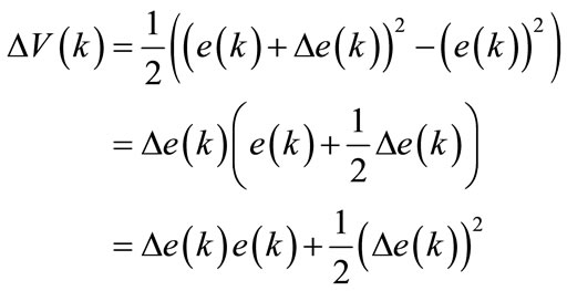
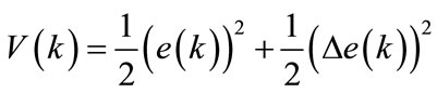
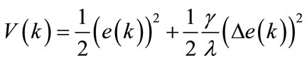
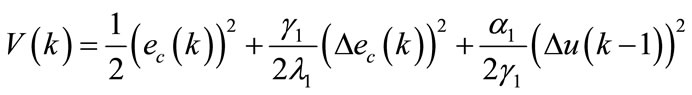
The first candidate Lyapunov function is defined by:
 (21)
(21)
The function  satisfies the following conditions:
 is continuous and differentiable.
 si
si  .
.
 ,
,  .
.
The neural model is stable in the sense of Lyapunov if  or simply
  .
.
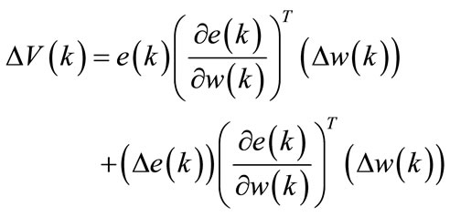
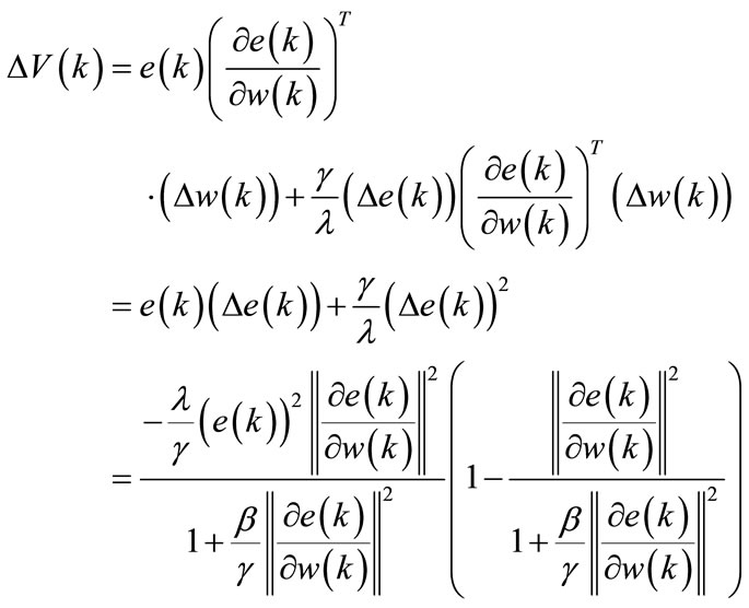
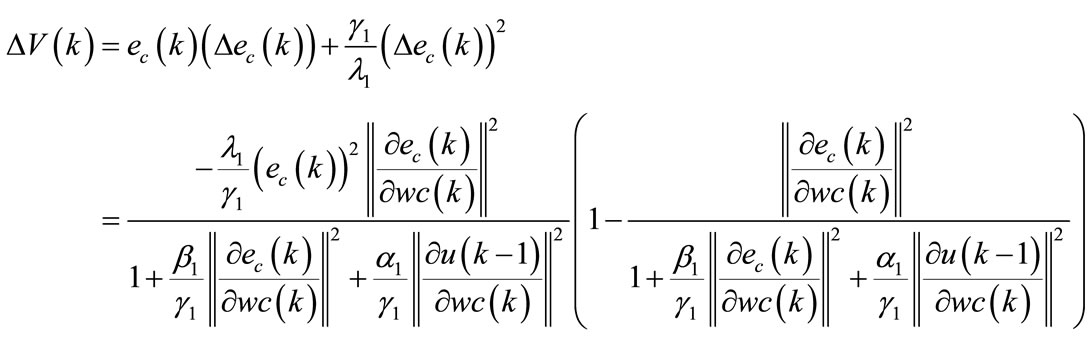
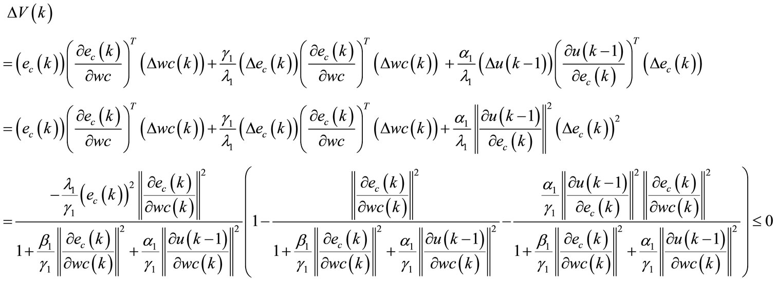
The term  is given by the following equation:
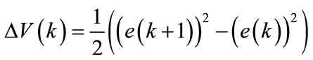 (22)
(22)
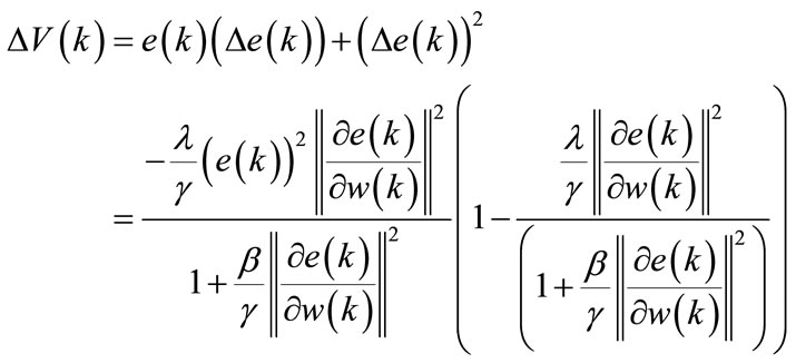
From Equation (22),  may be as follows:
 (23)
(23)
From the above equations, we obtain:
 (24)
(24)
like:
 (25)
(25)
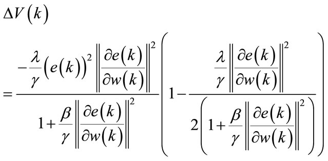
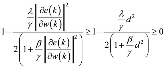
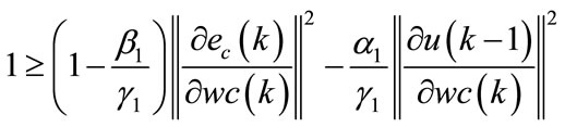
The proposed neural model is stable in the sense of Lyapunov if and only if:
 (26)
(26)
noting that:
 (27)
(27)
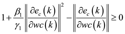
Therefore, we will have:
 (28)
(28)
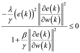
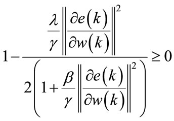
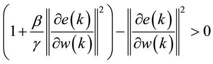
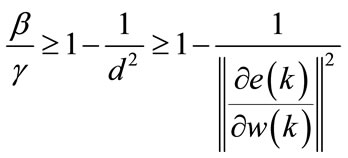
The stability condition becomes:
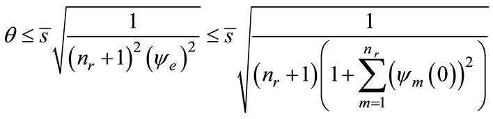
 (29)
(29)
The second candidate Lyapunov function is:
 (30)
(30)
Given that:
 (31)
(31)
Using Equations (19) and (20), the above relation becomes:
 (32)
(32)
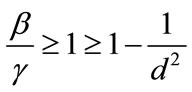
Then the second stability condition is:
 (33)
(33)
The third and last candidate Lyapunov function is:
 (34)
(34)
The term  is as follows:
 (35)
(35)
The third stability condition is:
 (36)
(36)
therefore:
 (37)
(37)
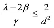
To meet the three conditions of stability of Lyapunov candidate functions proposed parameters ,
,  and
and  must verify:
 (38)
(38)
 (39)
(39)
then:
 (40)
(40)
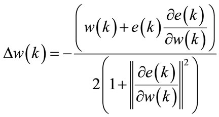
Theorem 2. The parameters of the neural network can be adjusted using the following equation:
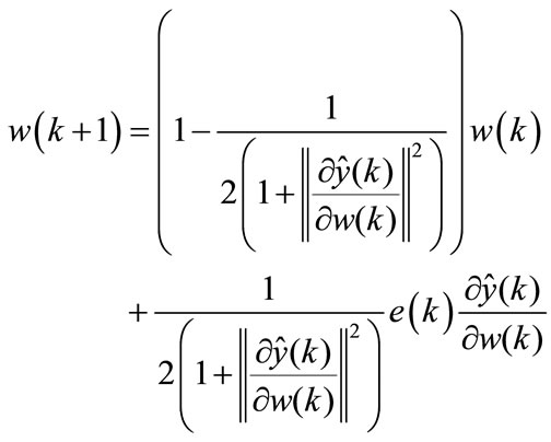 (41)
(41)
Proof:
Using the following Lyapunov function:
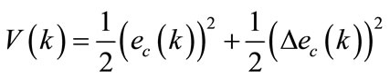
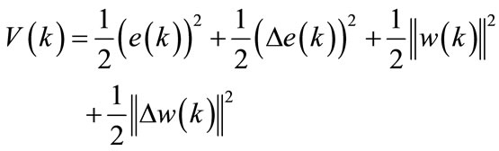 (42)
(42)
The learning procedure of the neural network is stable if:
 (43)
(43)
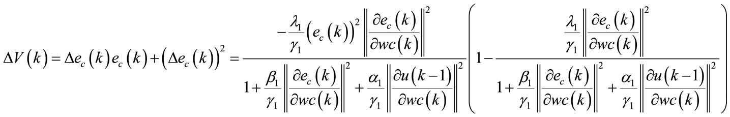
Using the above equation, we can write:
 (44)
(44)
such as 
therefore:
 (45)
(45)
For Equation (45) has a unique solution requires that:
 (46)
(46)
then:
 (47)
(47)
The term  can be written as follows:
 (48)
(48)
For a very small variation, we can write Equation (48):
 (49)
(49)
therefore:
 (50)
(50)
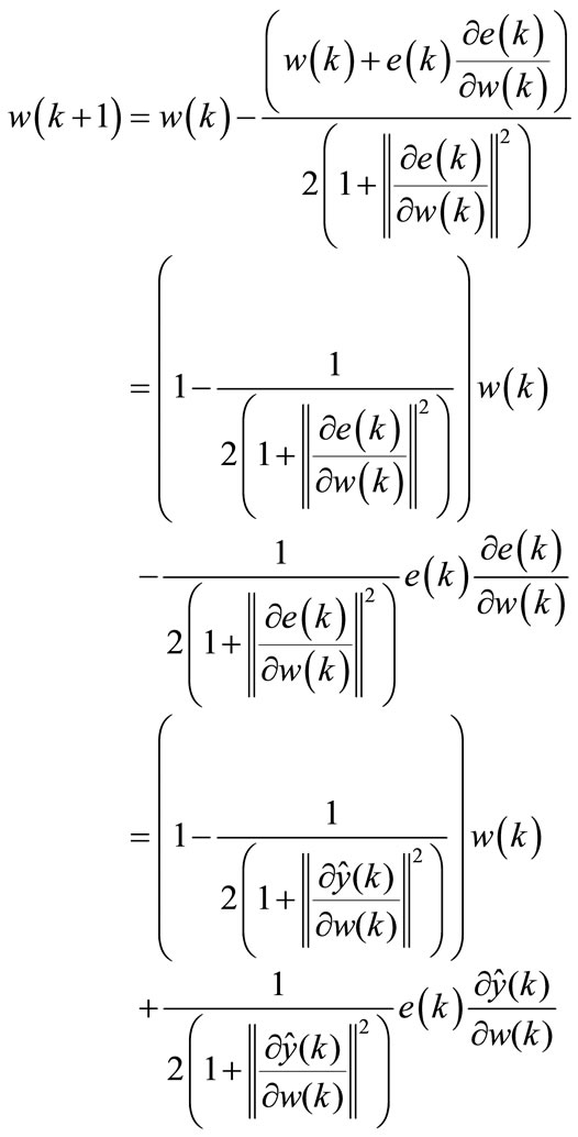
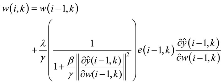
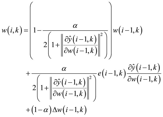
Theorem 3. The updating of the neural network parameters can be made by the following equation:
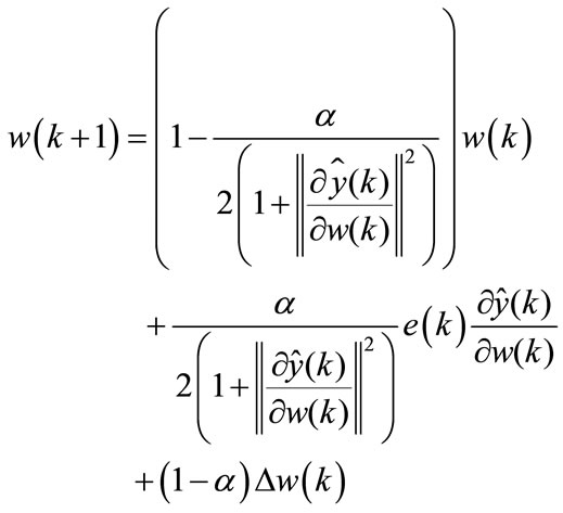 (51)
(51)
with: 
Proof:
From Equations (14) and (41), we can write:
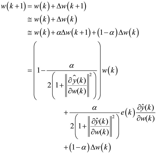 (52)
(52)
The choice of initial synaptic weights and biases can affect the speed of convergence of the learning algorithm of the neural network [36-47]. According to [48], the weights can be initialized by a random number generator with a uniform distribution between  and
and  or a normal distribution
  .
.
For weights with uniform distribution:
 (53)
(53)
For weight with a normal distribution:
 (54)
(54)
where: 
2.3. Organizational of the Learning Algorithm of Neural Model
The proposed Lyapunov-Based used to training dynamic model of the system is presented by the flowchart in Figure 2, reads as follows:
Step 1:
We fix the desired square error  , the parameters
  , the number of samples
  , the maximum number of iterations
 , the number of neurons in the first hidden layer
  .
.
The weights  are initialized by a random number generator with a normal distribution between
  and
and  .
.
where:
 (55)
(55)
 (56)
(56)
Initialize:
- the output of the neural network
 (57)
(57)
- the vector of outputs of the hidden layer:
 (58)
(58)
- the vector potentials of neurons in the hidden layer:
 (59)
(59)
- the input vector of the neural network:
 (60)
(60)
Step 2:
initialize:
 (61)
(61)
 (62)
(62)
 (63)
(63)
 (64)
(64)
Step 3:
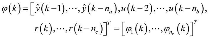
Consider an input vector network
and the desired value for output .
.
Step 4:
Calculate the output of the neural network  .
.
Step 5:
Calculate the difference between the system output and the model  .
.
Step 6:
Calculate the square error  .
.
Step 7:
Adjust the vector of network parameters  using one of the three following relations:
 (65)
(65)
 (66)
(66)
with 
 (67)
(67)
with 
Step 8:
If the number of iterations  or
or  , proceed to Step 9.
Otherwise, increment i and return to Step 4.
Step 9:
Save:
- the weights of the network at time  :
:
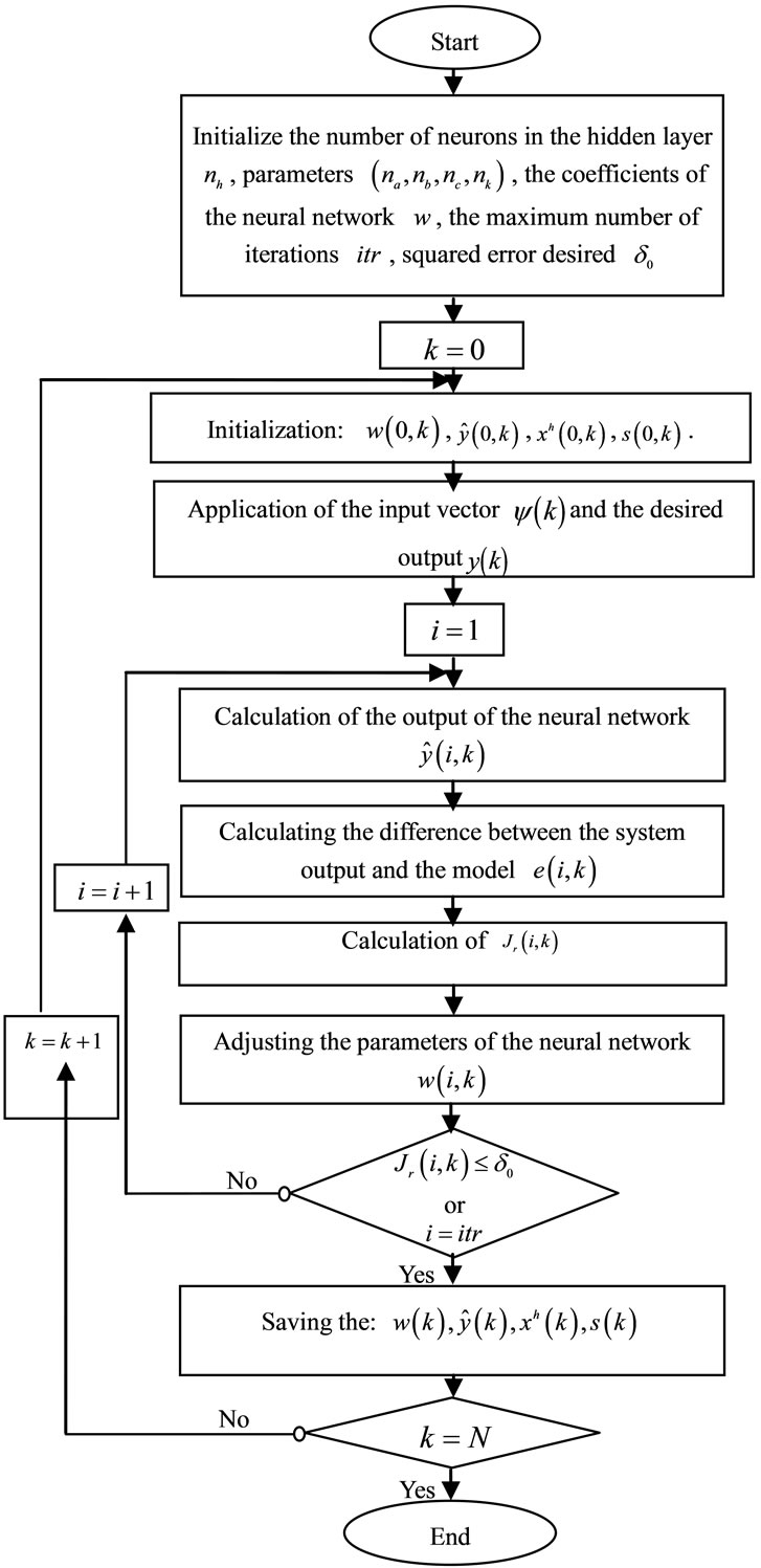
Figure 2. Flowchart of the learning algorithm of the neural network.
 (68)
(68)
- the output of the neural network:
 (69)
(69)
- the vector of outputs of the hidden layer:
 (70)
(70)
- the vector potentials of neurons in the hidden layer:
 (71)
(71)
Step 10:
If  , proceed to Step11.
Otherwise, increment and return to Step 2.
Step 11:
Stop learning.
The flowchart of this algorithm is given in Figure 2.
2.4. Validation Tests of the Neuronal Model
The neuronal model obtained from the estimation of its parameters is valid strictly used for the experiment. So check it is compatible with other forms of input in order to properly represent the system operation to identify. Most static tests of model validation are based on the criterion of Nash, on the auto-correlation of residuals, based on cross-correlation between residues and other inputs to the system. According to [49], the Nash criterion is given by the following equation:
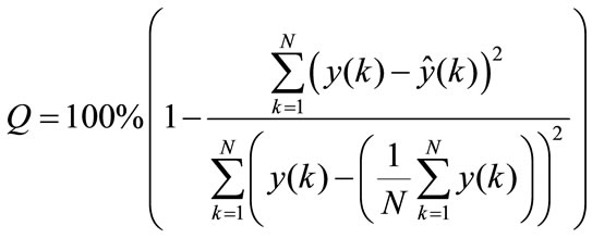 (72)
(72)
N is the number of samples.
In [50-52], the correlation functions are:
- autocorrelation function of residuals:
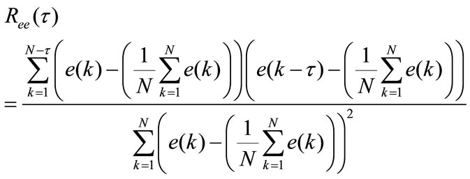 (73)
(73)
- crosscorrelation function between the residuals and the previous entries:
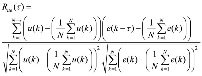 (74)
(74)
Ideally, if the model is validated, the results of correlation tests and the Nash criterion following results:
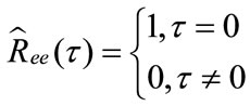 ,
, 
 and
and .
.
Typically, we verify that  and the functions
  are null for the interval
  with a confidence interval 95%, that is to say that:
 .
.
3. Adaptive Control of Complex Dynamic Systems
In this section, we propose a structure of neural adaptive control of a complex dynamic system and three learning algorithms of a neuronal controller.
3.1. Structure of the Proposed Adaptive Control
In this work, the architecture of the proposed adaptive control is given in Figure 3.
The considered neural network is first trained off-line to learn the inverse dynamics of the considered system from the input-output data. The model following adaptive control approach is performed after the training process is achieved. The proposed Lyapunov-Base training algorithm is used to adjust the considered neural network weights so that the neural model output follows the desired one.
3.2. Learning Algorithms of Neural Controller
Three learning algorithms of the neural controller are proposed.
Theorem 4. Learning the neuronal controller may be effected by the following equation:
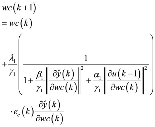 (75)
(75)
with:
 (76)
(76)
 (77)
(77)
 is the reference signal.
 (78)
(78)
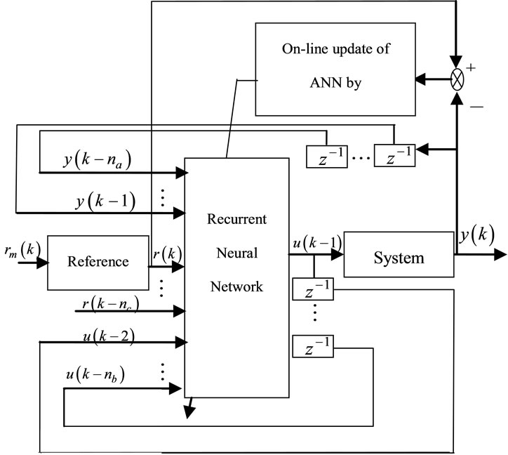
Figure 3. Structure of the proposed adaptive control.
are the weight of the neuronal controller.
Proof:
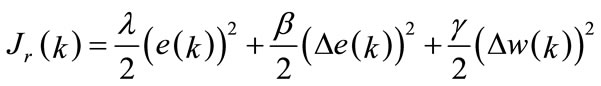
The control system consists of using an optimization digital non-linear algorithm to minimize the following criterion:
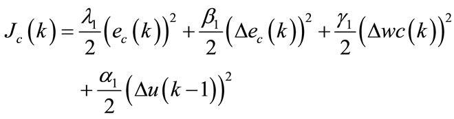 (79)
(79)
with:
 (80)
(80)
 (81)
(81)
 (82)
(82)
 (83)
(83)
 (84)
(84)
 (85)
(85)
 (86)
(86)
 (87)
(87)
The minimum of criterion  is reached when:
 (88)
(88)
The solution of Equation (88) calculates the weight of the neuronal controller as follows:
 (89)
(89)
The term  defined by:
 (90)
(90)
therefore:
 (91)
(91)
Using the above equations, the relationship giving the vector  minimizing the criterion
  can be written as follows:
 (92)
(92)
It is necessary to check the stability of this procedure to adjust the weight of the correction before applying. In this case, the candidate Lyapunov function may be as follows:
 (93)
(93)
According to Equation (32), the term  is written as follows:
 (94)
(94)
For the procedure to adjust the parameters of the controller is stable, it must:
 (95)
(95)
then:
 (96)
(96)
The second condition for stability is obtained by the following Lyapunov function:
 (97)
(97)
From the Equation (35), we can write:
 (98)
(98)
The learning algorithm parameters of the controller are stable if:
 (99)
(99)
Using the following Lyapunov function:
 (100)
(100)
The adjustment procedure is stable if the parameters:
 (101)
(101)
The third stability condition is:
 (102)
(102)
Assuming:
 (103)
(103)
 (104)
(104)
Therefore:
 (105)
(105)
The fourth condition for stability is obtained by the following Lyapunov function:
 (106)
(106)
The term  is as follows:
 (107)
(107)
For the learning algorithm is stable, it must:
 (108)
(108)
therefore:
 (109)
(109)
According to Equations (96), (105) and (109), we can write:
 (110)
(110)
The stability conditions can be so:
 (111)
(111)
The term  is calculated by the following equations:
 (112)
(112)
 (113)
(113)
 (114)
(114)
Theorem 5. The procedure for adjusting the parameters of neuronal controller can be described by the following equation:
 (115)
(115)
Proof:
From the following Lyapunov function:
 (116)
(116)
The procedure for adjusting the parameters of the neuronal controller is stable if:
 (117)
(117)
such as: 
Equation (117) becomes:
 (118)
(118)
If the above equation has a unique solution, the term  is as follows:
 (119)
(119)
The equation for adjusting the parameters of the neuronal controller can be written:
 (120)
(120)
therefore:
 (121)
(121)
Theorem 6. The procedure for adjusting controller parameters can be made by the following equation:
 (122)
(122)
Proof:
Using the Equation (121), we may write:
 (123)
(123)
Flowchart of the learning algorithm of the neural controller Once the modeling phase is completed, the calculation of parameters of neuronal controller is carried through the following steps:
Step 1:
We fix the desired square error  , the parameters
  , the number of samples N, the maximum number of iterations
  , the number of neurons in the hidden layer
  .
.
The weights are initialized by a random number generator with a normal distribution between
  and
and  .
.
where:
 (124)
(124)
with:
 (125)
(125)
Step 2:
Initialize:
 (126)
(126)
 (127)
(127)
 (128)
(128)
 (129)
(129)
Step 3:
Consider an input vector of the network

and the reference signal .
.
Step 4:
Calculate the output of the neuronal controller  .
.
Step 5:
Calculate the output of the neural model  .
.
Step 6:
Calculating the difference between the reference signal and the output of neural model  .
.
Step 7:
Calculate the square error  .
.
Step 8:
Adjust the vector of network parameters  using one of the three following relations:
 (130)
(130)
 (131)
(131)
with ,
,  ,
, 
 (132)
(132)
Step 9:
If the number of iterations  or
or  , proceed to Step 10.
Otherwise, increment and return to Step 4.
Step 10:
Save:
- the weights of the network at time  :
:
 (133)
(133)
- the output of the neuronal controller:
 (134)
(134)
- the vector of outputs of the hidden layer:
 (135)
(135)
- the vector potentials of neurons in the hidden layer:
 (136)
(136)
Step 11:
If  , proceed to Step 12.
Otherwise, increment  and return to Step 2.
Step 12:
Stop Learning.
These steps are represented by the following flowchart, Figure 4.
4. Numerical Results and Discussion
Let consider the nonlinear system described by the following equation of state:
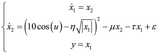 (137)
(137)

Figure 4. Flowchart of the proposed Lyapunov-Base learning algorithm of the controller neural network.
with:
 and
and  are respectively the input and output system.
 is a noise such as
 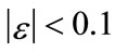 .
.
The Figure 5 shows the evolution of system parameters
( ,
, and
and ).
).
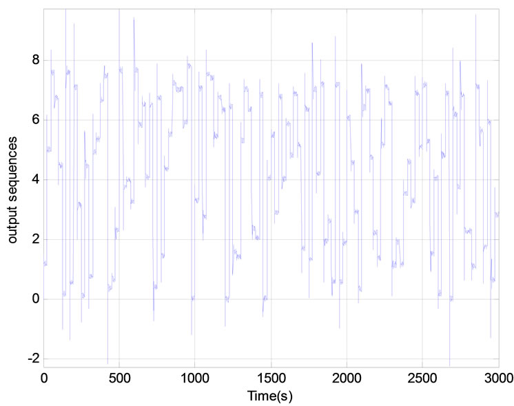
The sequences of input and output those used to calculate the parameters of the neural model are shown in Figure 6. These sequences show the system response to
 (a)
(a)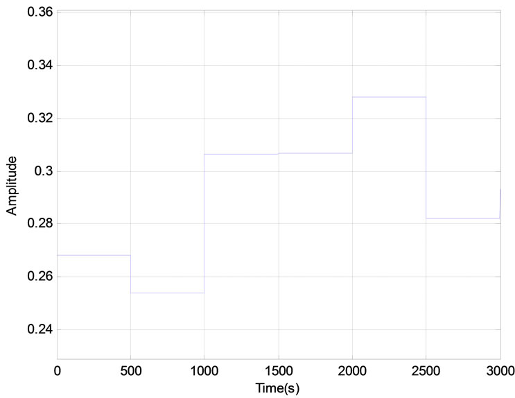 (b)
(b) (c)
(c)
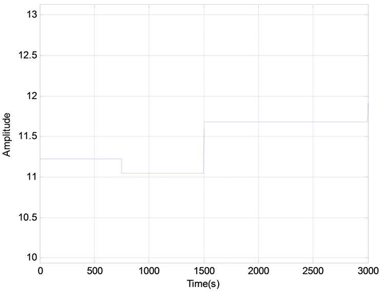
Figure 5. Evolution of the system parameters: (a) parameter η; (b) parameter τ; (c) parameter μ.
 (a)
(a)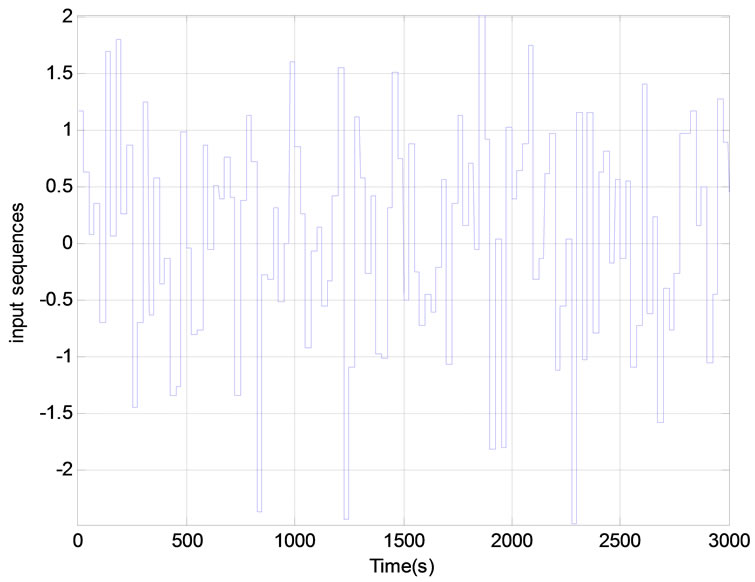 (b)
(b)
Figure 6. Training data-pattern: (a) input sequences; (b) output sequences.
 (a)
(a)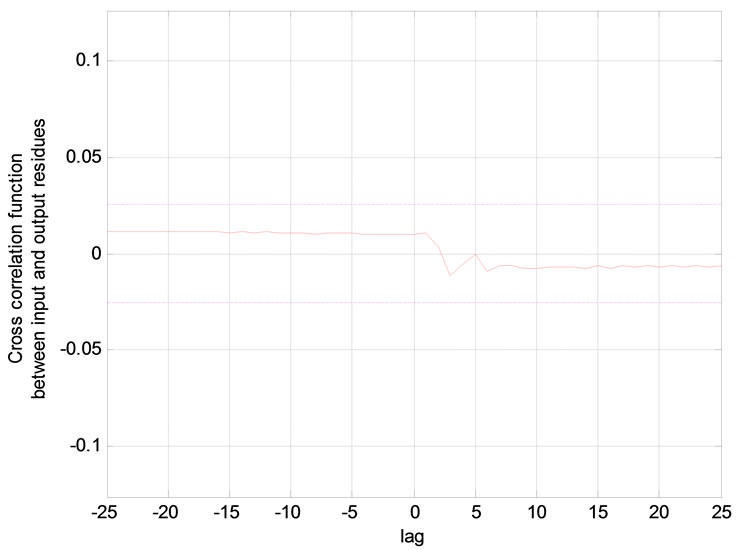 (b)
(b)
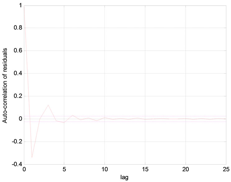
Figure 7. Validation tests of the model: (a) Auto-correlation of residuals; (b) Cross correlation function between input and output residues.
 (a)
(a)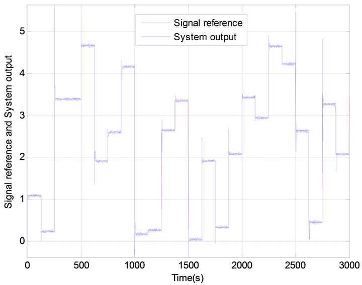 (b)
(b)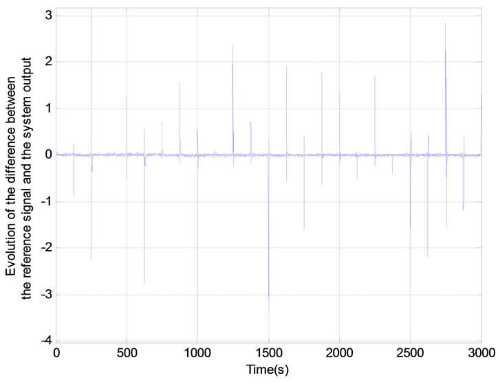 (c)
(c)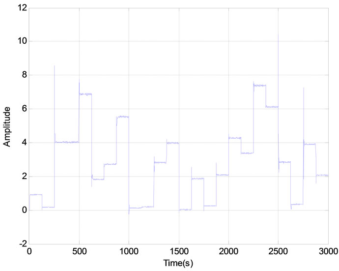 (d)
(d)
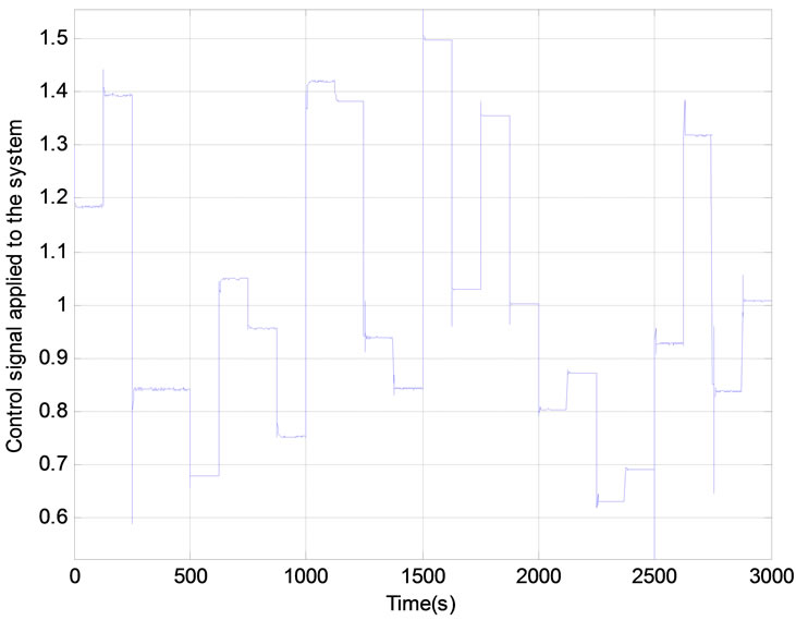
Figure 8. Results of adaptive control system in the case of a reference signal amplitude random uniform distribution: (a) Control signal applied to the system; (b) Response of the system; (c) Evolution of the difference between the reference signal and the system output; (d) Sensitivity of the process.
 (a)
(a)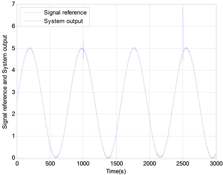 (b)
(b)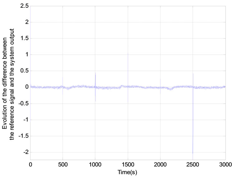 (c)
(c)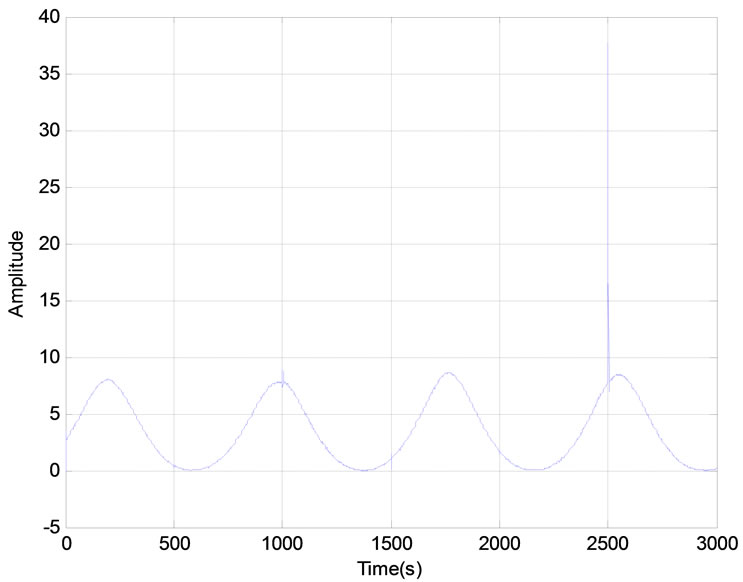 (d)
(d)
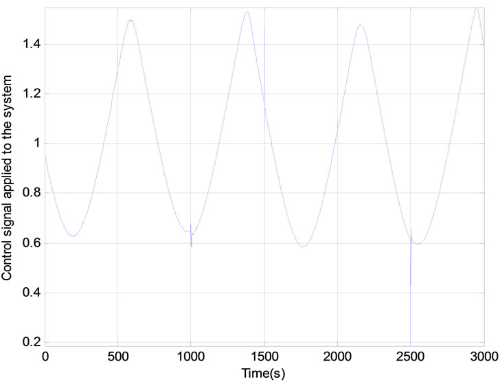
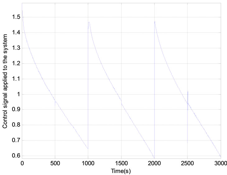
Figure 9. Results of adaptive control system in the case of a sinusoidal reference signal: (a) Control signal applied to the system; (b) Response of the system; (c) Evolution of the difference between the reference signal and the system output; (d) Sensitivity of the process.
 (a)
(a)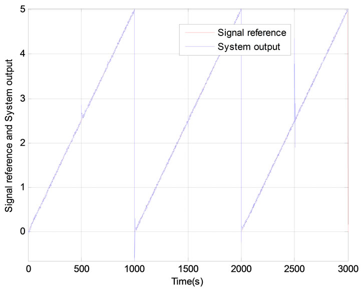 (b)
(b) (c)
(c)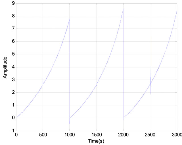 (d)
(d)
Figure 10. Results of adaptive control system in the case of a triangular reference signal: (a) Control signal applied to the system; (b) Response of the system; (c) Evolution of the difference between the reference signal and the system output; (d) Sensitivity of the process.
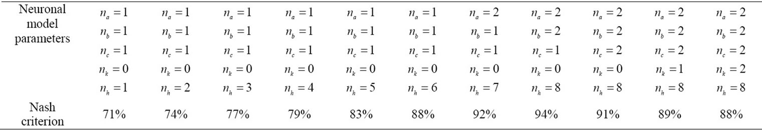
Table 1. Values of the Nash criterion of candidate neural models using Theorem 1 with (λ = 1, β = γ = 2).

Table 2. Values of the Nash criterion of candidate neural models using Theorem 2.

Table 3. Values of the Nash criterion of candidate neural models using Theorem 3 (α = 0.7).
a random signal of zero mean and variance 1.
The evolution of the Nash criterion of different candidate models of the system (Tables 1-3) can be concluded that ,
,  ,
,  ,
,  ,
,  , 8 neurons in the hidden layer use of Theorem 3 for the learning phase, is necessary and sufficient for a neuronal model of a satisfactory precision.
The autocorrelation functions of residuals and crosscorrelation between input and residuals (Figure 7) are within the confidence intervals, thus validating the use of the network chosen as a model of the system studied.
After the learning phase of the neuronal model completed, the structure proposed of neural adaptive control is applied to the system. In this case, the learning algorithm of the neural controller uses Theorem 6. The results are presented in Figures 8, 9 and 10. It appears from these figures that this control strategy provides satisfactory results. Indeed, the system follows the reference signal appropriately by responding to the objectives: rejection of disturbances, the control performance, robustness and system stability.
5. Conclusion
In this paper, we have proposed adaptive control structure for a complex dynamic system using a recurrent neural network. Before, the application of the proposed adaptive neuro control, the recurrent neural has been trained off-line to implement the inverse dynamic of the considered system using a proposed Lyapunov-Base system training algorithm. The simulation results obtained show the effectiveness of the recurrent neural network structure and its adaptation algorithm to simulate the inverse dynamics of the system, and to control it in closed loop with good tracking performance.
REFERENCES
- L. J. Chen and K. S. Narendra, “Nonlinear Adaptive Control Using Neural Networks and Multiple Models,” Automatica, Vol. 37, No. 8, 2001, pp. 1245-1255. doi:10.1016/S0005-1098(01)00072-3
- A. Bagheri, T. Karimi and N. Amanifard, “Tracking Performance Control of a Cable Communicated Underwater Vehicle Using Adaptive Neural Network Controllers,” Applied Soft Computing, Vol. 10, No. 3, 2001, pp. 908- 918. doi:10.1016/j.asoc.2009.10.008
- D. L. Yu, T. K. Chang and D. W. Yu, “Adaptive Neural Model-Based Fault Tolerant Control for Multi-Variable Processes,” Engineering Applications of Artificial Intelligence, Vol. 18, No. 4, 2005, pp. 393-411. doi:10.1016/j.engappai.2004.10.003
- J. M. Renders, “Algorithmes Génétiques et Réseaux de Neurones,” Hermes Sciences Publicat, Paris, 1995.
- Y.-K. Choi, M.-J. Lee, S. Kim and Y.-C. Kay, “Design and Implementation of an Adaptive Neural Network Compensator for Control Systems,” IEEE Transactions on Industrial Electronics, Vol. 48, No. 2, 2001, pp. 416- 423. doi:10.1109/41.915421
- N. Magnus, et al., “Neural Networks for Modelling and Control of Dynamic Systems,” Springer Berlin, Heidelberg, 2000.
- I. Kar and L. Behera, “Direct Adaptive Neural Control for Affine Nonlinear Systems,” Applied Soft Computing, Vol. 9, No. 2, 2009, pp. 756-764. doi:10.1016/j.asoc.2008.10.001
- F. N. Koumboulis and N. D. Kouvakas, “Indirect Adaptive Neural Control for Precalcination in Cement Plants,” Mathematics and Computers in Simulation, Vol. 60, No. 3-5, 2002, pp. 325-334. doi:10.1016/S0378-4754(02)00024-1
- Z. Nagy, S. Agachi and L. Bodizs, “Adaptive Neural Network Model Based Nonlinear Predictive Control of a Fluid Catalytic Cracking Unit,” Computer Aided Chemical Engineering, Vol. 8, 2000, pp. 235-240. doi:10.1016/S1570-7946(00)80041-3
- T. T. Hu, J. H. Zhu and Z. Q. Sun, “Robust Adaptive Neural Control of a Class of MIMO Nonlinear Systems,” Tsinghua Science & Technology, Vol. 12, No. 1, 2007, pp. 14-21. doi:10.1016/S1007-0214(07)70003-2
- H. Deng, H. X. Li and Y. H. Wu, “Feedback-LinearizationBased Neural Adaptive Control for Unknown Nonaffine Nonlinear Discrete-Time Systems,” IEEE Transactions on Neural Networks, Vol. 19, No. 9, 2008, pp. 1615-1625.
- C. J. Yu, J. H. Zhu and Z. Q. Sun, “Adaptive Neural Network Internal Model Control for Tilt Rotor Aircraft Platform,” Advances in Natural Computation, Vol. 3611, 2005, pp. 262-265. doi:10.1007/11539117_38
- S. Yang, W. Q. Qian, W. S. Yan and J. Li, “Adaptive Depth Control for Autonomous Underwater Vehicles Based on Feedforward Neural Networks,” International Journal of Computer Science & Applications, Vol. 4, No. 3, 2007, pp. 107-118.
- M. Jalali-Heravi, M. Asadollahi-Baboli and P. Shahbazikhah, “QSAR Study of Heparanase Inhibitors Activity Using Artificial Neural Networks and Levenberg-Marquardt Algorithm,” European Journal of Medicinal Chemistry, Vol. 43, No. 3, 2008, pp. 548-556. doi:10.1016/j.ejmech.2007.04.014
- K.-I. Funahashi, “On the Approximate Realization of Continuous Mapping by Neural Networks,” Neural networks, Vol. 2, No. 3, 1989, pp. 183-192. doi:10.1016/0893-6080(89)90003-8
- G. Cybenko, “Approximation by Superposition of a Sigmoidal Function,” Mathematics of Control, Signal, and Systems, Vol. 2, 1989, pp. 303-314.
- D. Psaltis, A. Sideris and A. A. Yamamura, “A Multilayered Neural Network Control,” IEEE Control Systems Magazine, Vol. 8, No. 2, 1988, pp. 17-21. doi:10.1109/37.1868
- J. Baltersee and J. A. Chambers, “Nonlinear Adaptive Prediction of Speech with a Pipelined Recurrent Neural Network,” IEEE Transactions on Signal Processing, Vol. 46, No. 8, 1998, pp. 2207-2216. doi:10.1109/78.705435
- D. G. Stavrakoudis and J. B. Theocharis, “Pipelined Recurrent Fuzzy Neural Networks for Nonlinear Adaptive Speech Prediction,” IEEE Transactions on Systems, Man, and Cybernetics, (Part B): Cybernetics, Vol. 37, No. 5, 2007, pp. 1305-1320. doi:10.1109/TSMCB.2007.900516
- H. Q. Zhao and J. S. Zhang, “A Novel Adaptive Nonlinear Filter Based Pipelined Feedforward Second-Order Volterra Architecture,” IEEE Transactions Signal Processing, Vol. 57, No. 1, 2009, pp. 237-246. doi:10.1109/TSP.2008.2007105
- P.-R. Chang and J.-T. Hu, “Optimal Nonlinear Adaptive Prediction and Modeling of MPEG Video in ATM Networks Using Pipelined Recurrent Neural Networks,” IEEE Journal of Selected Areas in Communications, Vol. 15, No. 6, 1997, pp. 1087-1100. doi:10.1109/49.611161
- Y.-S. Chen, C.-J. Chang and Y.-L. Hsieh, “A Channel Effect Prediction-Based Power Control Scheme Using PRNN/ERLS for Uplinks in DS-CDMA Cellular Mobile Systems,” IEEE Transactions on Wireless Communications, Vol. 5, No. 1, 2006, pp. 23-27. doi:10.1109/TWC.2006.1576521
- D. P. Mandic and J. A. Chambers, “Toward an Optimal PRNN-Based Nonlinear Prediction,” IEEE Transactions on Neural Networks, Vol. 10, No. 6, 1999, pp. 1435-1442. doi:10.1109/72.809088
- D. P. Mandic and J. A. Chambers, “On the Choice of Parameters of the Cost Function in Nested Modular RNN’s,” IEEE Transactions on Neural Networks, Vol. 11, No. 2, 2000, pp. 315-322. doi:10.1109/72.839003
- H. Q. Zhao and J. S. Zhang, “Pipelined Chebyshev Functional Link Artificial Recurrent Neural Network for Nonlinear Adaptive Filter,” IEEE Transactions on Systems, Man, and Cybernetics Part B: Cybernetics, Vol. 40, No. 1, 2010, pp. 162-172. doi:10.1109/TSMCB.2009.2024313
- R. J. Williams and D. Zipser, “A Learning Algorithm for Continually Running Fully Recurrent Neural Networks,” Neural Computation, Vol. 1, No. 2, 1989, pp. 270-280. doi:10.1162/neco.1989.1.2.270
- B. A. Pearlmutter, “Dynamic Recurrent Neural Networks,” Technical Report CMU-CS-88-191, Information Science and Technology Office, 1990.
- B. A. Pearlmutter, “Gradient Calculations for Dynamic Recurrent Neural Networks: A Survey,” IEEE Transactions on Neural Networks, Vol. 6, No. 5, 1995, pp. 1212- 1228. doi:10.1109/72.410363
- H. Al-Duwaish, M. N. Karim and V. Chandrasekar, “Use of Multilayer Feedforward Neural Networks in Identification and Control of Wiener Model,” IEEE Proceedings— Control Theory and Applications, Vol. 143, No. 3, 1996, pp. 255-258. doi:10.1049/ip-cta:19960376
- K. S. Narendra and K. Parthasarathy, “Identification and Control of Dynamical Systems Using Neural Networks,” IEEE Transactions on Neural Networks, Vol. 1, No. 1, 1990, pp. 4-27. doi:10.1109/72.80202
- C.-C. Ku and K. Y. Lee, “Diagonal Recurrent Neural Networks for Dynamic Systems Control,” IEEE Transactions on Neural Networks, Vol. 6, No. 1, 1995, pp. 144-156. doi:10.1109/72.363441
- H. Chaoui and P. Sicard, “Adaptive Lyapunov-Based Neural Network Sensorless Control of Permanent Magnet Synchronous Machines,” Neural Computing & Applications, Vol. 20, No. 5, 2010, pp. 717-727. doi:10.1007/s00521-010-0412-6
- R. A. Hooshmand and G. Isazadeh, “Application of Adaptive Lyapunov-Based UPFC Supplementary Controller by Neural Network Algorithm in Multi-Machine Power System,” Electrical Engineering (Archiv fur Elektrotechnik), Vol. 91, No. 4-5, 2009, pp. 187-195. doi:10.1007/s00202-009-0132-z
- T. Yabuta and T. Yamada, “Learning Control Using Neural Networks,” Proceedings of 1991 IEEE International conference on Robotics and Automation, Sacramento, 9- 11 April 1991, pp. 740-745. doi:10.1109/ROBOT.1991.131673
- Y. H. Tan and A. van Cauwenberghe, “Nonlinear OneStep-Ahead Control Using Neural Networks: Control Strategy and Stability Design,” Automatica, Vol. 32, No. 12, 1996, pp. 1667-1667. doi:10.1016/S0005-1098(96)80006-9
- T. Denoeux and R. Lengellé, “Initializing Back Propagation Networks with Prototypes,” Neural Networks, Vol. 6, No. 3, 1993, pp. 351-363. doi:10.1016/0893-6080(93)90003-F
- G. P. Drago and S. Ridella, “Statistically Controlled Activation Weight Initialization (SCAWI),” IEEE Transactions on Neural Networks, Vol. 3, No. 4, 1992, pp. 627- 631. doi:10.1109/72.143378
- J.-P. Martens, “A Stochastically Motivated Random Initialization of Pattern Classifying MLPs,” Neural Processing Letters, Vol. 3, No. 1, 1996, pp. 23-29. doi:10.1007/BF00417786
- T. Masters, “Practical Neural Network Recipes in C++,” Academic Press, Boston, 1993.
- D. Nguyen and B. Widrow, “Improving the Learning Speed of 2-Layer Neural Networks by Choosing Initial Values of the Adaptive Weights,” 1990 IJCNN International Joint Conference on Neural Networks, San Diego, 17-21 June 1990, pp. 21-26. doi:10.1109/IJCNN.1990.137819
- S. Osowski, “New Approach to Selection of Initial Values of Weights in Neural Function Approximation,” Electronics Letters, Vol. 29, No. 3, 1993, pp. 313-315. doi:10.1049/el:19930214
- J. F. Shepanski, “Fast Learning in Artificial Neural Systems: Multilayer Perceptron Training Using Optimal Estimation,” 1998 IEEE International Conference on Neural Networks, San Diego, 24-27 July 1988, pp. 465-472. doi:10.1109/ICNN.1988.23880
- H. Shimodaira, “A Weight Value Initialization Method for Improving Learning Performance of the Back Propagation Algorithm in Neural Networks,” 1994 Proceedings of Sixth International Conference on Tools with Artificial Intelligence, New Orleans, 6-9 November 1994, pp. 672- 675. doi:10.1109/TAI.1994.346429
- Y. F. Yam and T. W. S. Chow, “Determining Initial Weights of Feedforward Neural Networks Based on Least Squares Method,” Neural Processing Letters, Vol. 2, No. 2, 1995, pp. 13-17. doi:10.1007/BF02312350
- Y. F. Yam, T. W. S. Chow and C. T. Leung, “A New Method in Determining Initial Weights of Feedforward Neural Networks for Training Enhancement,” Neurocomputing, Vol. 16, No. 1, 1997, pp. 23-32. doi:10.1016/S0925-2312(96)00058-6
- L. F. A. Wessels and E. Barnard, “Avoiding False Local Minima by Proper Initialization of Connections,” IEEE Transactions on Neural Networks, Vol. 3, No. 6, 1992, pp. 899-905. doi:10.1109/72.165592
- N. Weymaere and J.-P. Martens, “On the Initialization and Optimization of Multilayer Perceptrons,” IEEE Transactions on Neural Networks, Vol. 5, No. 5, 1994, pp. 738- 751. doi:10.1109/72.317726
- J. Y. F. Yam and T. W. S. Chow, “A Weight Initialization Method for Improving Training Speed in Feedforward Neural Network,” Neurocomputing, Vol. 30, No. 1-4, 2000, pp. 219-232. doi:10.1016/S0925-2312(99)00127-7
- J. E. Nash and J. V. Sutcliffe, “River Flow Forecasting through Conceptual Models Part I—A Discussion of Principles,” Journal of Hydrology, Vol. 10, No. 3, 1970, pp. 282-290. doi:10.1016/0022-1694(70)90255-6
- S. A. Billings and Q. M. Zhu, “Nonlinear Model Validation Using Correlation Tests,” International Journal of Control, Vol. 60, No. 6, 1994, pp. 1107-1120. doi:10.1080/00207179408921513
- S. A. Billings, H. B. Jamaluddin and S. Chen, “Properties of Neural Networks with Applications to Modelling NonLinear Dynamical Systems,” International Journal of Control, Vol. 55, No. 1, 1992, pp. 193-224. doi:10.1080/00207179208934232
- F. Zouari, K. B. Saad and M. Benrejeb, “Adaptive Internal Model Control of DC-Motor Drive System Using Dynamic Neural Network,” Journal of Software Engineering and Applications, Vol. 5, No. 3, 2012, pp. 168-189. doi:10.4236/jsea.2012.53024
Appendixs
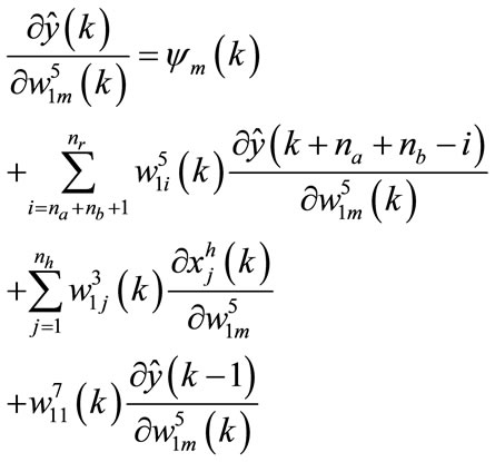
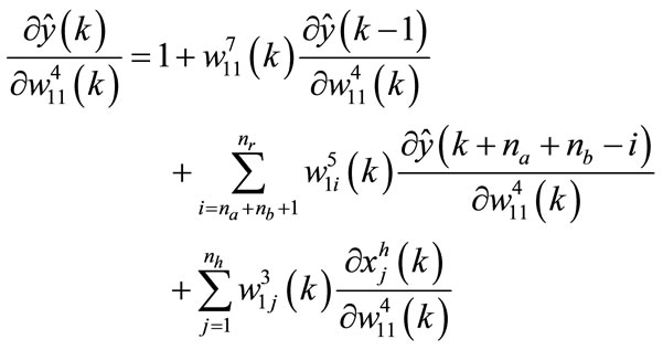
The calculation of the term  is performed by the following equations:
for the neuron in the output layer:
 (138)
(138)
 (139)
(139)
 (140)
(140)
 (141)
(141)
 (142)
(142)
 (143)
(143)
 (144)
(144)
 (145)
(145)
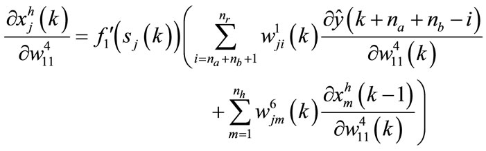
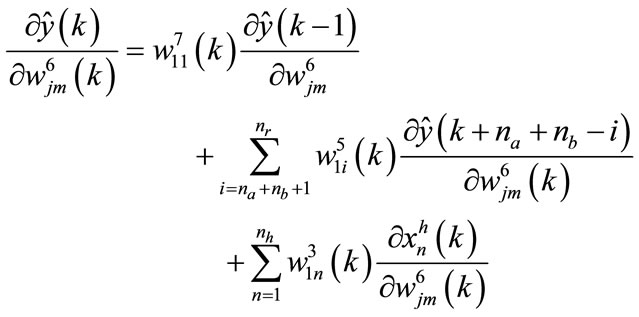
for a neuron in the hidden layer:
 (146)
(146)
 (147)
(147)

 (148)
(148)
 (149)
(149)

 (150)
(150)

 (151)
(151)
 (152)
(152)

 (153)
(153)
 (154)
(154)
From the above equations, we can write:
 (155)
(155)
 (156)
(156)
It was therefore:
 (157)
(157)
 (158)
(158)
 (159)
(159)
 (160)
(160)
 (161)
(161)
 (162)
(162)
 (163)
(163)