Journal of Biomedical Science and Engineering
Vol.5 No.9(2012), Article ID:22424,12 pages DOI:10.4236/jbise.2012.59062
About the structure of posturography: Sampling duration, parametrization, focus of attention (part I)
![]()
1Institute of Sport Sciences, Johann Wolfgang Goethe University, Frankfurt am Main, Germany
2Faculty of Health, Hochschule Fresenius, University of Applied Sciences, Idstein, Germany
Email: *p.schubert@sport.uni-frankfurt.de
Received 20 June 2012; revised 18 July 2012; accepted 30 July 2012
Keywords: Center of Pressure; Sample Duration; Posturographic Parameters; Exploratory Factor Analysis; Nonlinear Methods; Internal Focus of Attention
ABSTRACT
This study investigates the choice of posturographic parameter sets with respect to the influence of different sampling durations (30 s, 60 s, 300 s). Center of pressure (COP) data are derived from 16 healthy subjects standing quietly on a force plate. They were advised to focus on the postural control process (i.e. internal focus of attention). 33 common linear and 10 nonlinear parameters are calculated and grouped into five classes. Component structure in each group is obtained via exploratory factor analysis. We demonstrate that COP evaluation—irrespective of sampling duration—necessitates a set of diverse parameters to explain more variance of the data. Further more, parameter sets are uniformly invariant towards sampling durations and display a consistent factor loading pattern. These findings pose a structure for COP parametrization. Hence, specific recommendations are preserved in order to avoid redundancy or misleading basis for inter-study comparisons. The choice of 11 parameters from the groups is recommended as a framework for future research in posturography.
1. INTRODUCTION
Postural control is the ability to maintain the position of the body with respect to the environmental constraints especially gravitational effects. This feature is an omnipresent and essential part of everyday life activities principally during standing, sitting and even locomotion. The concise, comprehensive, valid and reliable assessment of postural control conduces to research evaluation, judgment and decision making in a clinical context. A simple method to derive pertinent experimental data is by measuring the centre of pressure (COP) on a force plate over time, which coincides with the vertical projection of the body’s center of mass [1]. Vertical standing posture requires the projection of the center of mass to be within an area that is proportional to the extent of the convex hull of the lateral borders of the feet, namely the base of support. When subjects are asked to stand as still as possible they never attain a stable equilibrium. Dealing with a multijoint segmented built-up and the resultant Bernsteinian problem of motor redundancy due to the amount of degrees of freedom, the organism is permanently exposed to an unstable condition which is observable in small motion of COP trajectories [2]. These fluctuations are believed to be regulated by a complex sensorimotor system [3-5]. Hence, investigating sway by means of COP displacements would deliver insight into neurophysiological processes and hints relevance for practical and theoretical applications. However, little success has been achieved in using posturography for discriminating quiet stance specifics [6]. The reason could be the lack of adequate standardization: e.g. the sampling duration, the measurement parameters [7], focus of attention (compare part II) [8-10]. First, measurement durations in research typically range from several seconds (e.g. [11,12]) up to 30 minutes [13-15]. With regard to clinical investigations sampling durations lower than 30 s are typical. However, it has been reported that sampling duration strongly affects the magnitudes of COP parameters [12,16]. On the one hand, prolonged standing conditions provoke specific postural events that modify postural performance [17,18]. On the other hand, COP migration is seen as a bounded nonstationary process and therefore short sampling durations (<60 s) do neither account for transient events nor for low frequency dynamics [19,20]. Second, a great variety of popsturographic parameters for COP description is available, which may as well assign a reason for contrary results in literature [21]. Concerning this matter Pavol (2005, p. 20) poses the questions “which measures best characterize postural sway, which measures are best for detecting differences in postural sway and how do differences in these measures relate to the postural control system?” [22]. It is widely accepted that multiple measures are needed to characterize postural fluctuations [21]. Recently, recommendations for the usage of descriptive parameters have been published by using principal component analysis [21,23]. However, one could conjecture the influence of sampling duration on the validity of descriptive posturographic parameter sets. The question whether different sampling times necessitate a different set of COP parameters is still left open. The present study investigates the influence of three different sampling durations (30 s, 60 s and 300 s) on the postural performance of quiet standing in healthy subjects with respect to the most common linear, but also more sophisticated nonlinear-parameters of posturography [24]. For this purpose, and with respect to earlier studies [21,23] a factor analysis approach is conducted to expose the sensitivity of different parameter groups to different measurement times.
Besides these basic research aspects, measuring postural control is of major interest in applied sciences. In rehabilitation, this procedure serves as a forecast instrument for a great amount of patients (e.g. orthopedic, neurologic, traumatological, etc.) or elderly subjects. However, COP data is often analyzed by only one parameter and therefore, results deal with limited significance. As a set of parameters will lead to more reasonable outcomes the present study provides a transfer for practical applications.
2. METHODS
2.1. Experimental Procedure
Sixteen healthy students (9 males and 7 females, age: 26.1 ± 6.7 years; height: 173.45 ± 11.14 cm; weight: 72.36 ± 13.04 kg) without musculoskeletal or neurological dysfunctions participated voluntarily in this study [24]. The subjects were instructed to stand with both feet parallel and upright as quiet as possible in hip width stance with arms relaxed at both sides while staring at a point on the wall in front and concentrating on the postural control process, which induces an internal focus of attention [8]. Three trials with different sampling durations (35 s, 65 s, 305 s) were conducted. 30 s is seen to be the typical clinical duration. At least 60 s is seen to be appropriate for time domain parameters, whereas the description of other parameters need 300 s of duration [7]. The experimental condition is referred to the typical laboratory condition and in practice, for example, to discriminate between different populations (e.g. [25]). Due to the fact that distance between the eyes and the visual field affects postural performance it was left unchanged during the whole measurement (about 2 m) [26]. Centre of pressure data (COP) were recorded by means of a 0.3
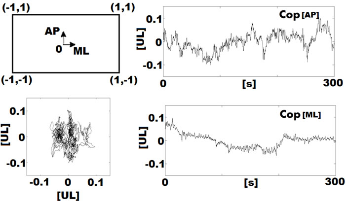
× 0.4 m2 force plate with a sampling rate of 1000 Hz. Subsequently, COP data were used to reckon anteriorposterior and medial-lateral movements labeled AP [unit of length: UL] and ML [UL] (Figure 1). A 4th order low-pass Butterworth filter with a cut-off frequency of 10 Hz was applied to eliminate measurement noise [1,27]. Next, time series were downsampled to 100 Hz (for calculation of entropy values to 20 Hz) and detrended by the mean of the time series. This procedure is appropriate for COP data as 95% of the informational content is within a range of the first Hertz [24,28]. Impact effects were eliminated by cutting the first 5 s from the time series. The person’s task temporally exceeded the measured samples so that no end effects were detectable.
2.2. Parameter Selection
Since, there exists no consent (if queried at all) which parameters should be chosen. For our purpose, we have selected the most common ones, which are typically used in the majority of medical research and practice. The different variables comprised traditional linear and nonlinear methods as proposed by diverse authors [24,28-31]. Duarte & Freitas (2010) subdivide the parameterization methods roughly into two groups: First, the traditional parameters which refer to estimations of the overall size
 (a)
(a)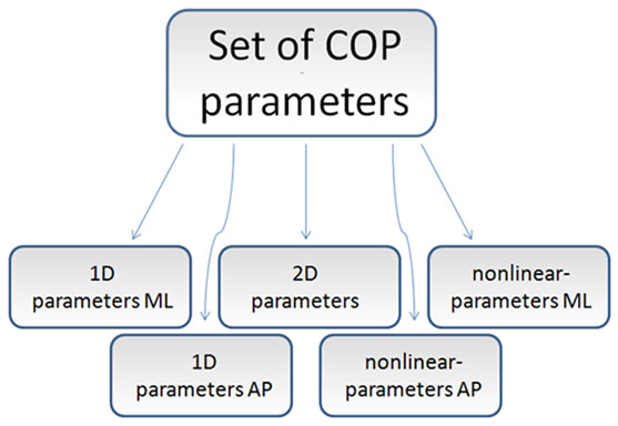 (b)
(b)
Figure 1. (a) Force plate and measurement directions. The COP position is expressed as a fraction of deviation from the midpoint of the force plate (values in units of length [UL]). Exemplary COP recording and resultant AP and ML time series; (b) Classification of COP parameters into five groups.
of COP excursions, second, structural posturographic and more sophisticated parameters which describe temporal pattern of the time series in a nonlinear manner [29]. The former ones are used as indicators of postural stability outlining COP displacements as random fluctuations. According to this theory, larger COP deflections are associated with less stable balance and in a next step with aging and disease. Consequently, the assumed random properties are treated as unwanted noise and averaged out. Temporal structures of the displacements are disregarded. In contrast, nonlinear methods determine the time-dependent structure of the time series. Against this background, both analysis techniques create complementary information [32,33].
Earlier studies recommend different procedures to attain a set of reliable parameters to evaluate the behavior of postural fluctuations. For instance, Kitibayashi et al. (2003) examined a large cohort of 220 subjects and found via factor analysis 4 factors that explained about two third of the total variance [23]. The factor structure is grouped into a unit time sway factor, mainly explained by velocity parameters, an AP sway factor, a ML sway factor and a frequency band power factor [34]. The authors suggest that parameters of these factors may synthetically characterize COP deflections. However, in their study nonlinear tools for COP evaluation were disregarded. Rocchi et al. (2004) calculated an amount of 37 stabilometric parameters [21]. Principal component analysis applied to 2-dimensional and 1-dimensional data separated in each case, identified 4 components on the one hand and 6 components on the other hand. In both categories the overall parameter loadings were similar, which corroborates the interdependent structure: size of the oscillation, spectral information and the relative weight of AP to ML components. This is in agreement to the findings of [30], and roughly to those of [23].
2.3. Traditional Parameters
Traditional parameters consist of values obtained in the time domain and frequency domain, which are also known as linear parameters [30]. Time domain describers are interrelated to either displacement of the COP or the velocity of the COP trace. Parameters of the frequency domain are associated with values calculated of the power spectral density (PSD) of the COP trace separated into an anterior-posterior (AP) and medio-lateral (ML) direction. A further classification which was achieved here alludes to the dimensionality of the calculated parameters. Time domain parameters can be subdivided into 1-dimensional (1D: AP and ML) or 2-dimensional (2D: COP trace) values whereas frequency parameters can only be calculated of 1-dimensional sequences.
Altogether, we calculated 33 traditional measures for the time domain and frequency domain time series via MATLAB© version 2008b routines in each experimental situation. In the time domain 5 parameters were included for 1D, each applied to AP and ML direction, and 13 parameters for 2D time series resulting in a sum of 23 values. In the frequency domain 5 parameters were computed respectively for AP and ML direction which compassed 10 different values. Table 1 summarizes these parameters.
We present a brief overview of those parameters for which the underlying algorithms are not immediately comprehensible. Otherwise, we state descriptive literature. A common procedure for COP evaluation is achieved by investigating the area covering the COP trace. Here, we used three different estimation approaches: 95% prediction ellipse, 95% prediction circumference and a convex hull method. A MATLAB© algorithm for the ellipse area is described e.g. in [29], where the coefficient of 2.4478 is the approximate value of the Chisquare distribution with 2 degrees of freedom (Figure 2). We are aware that the interpretation of the prediction ellipse is misleading; hence we refer to [29,30,35]. Circumference area was computed of the mean distance from the centre of the COP trajectory multiplied with the coefficient of 1.96 which represents the appropriate confidence region in the standard normal distribution. Both algorithms were useful to determine the estimated area of the COP deflections per second (see also [21]). The third method refers to the sector formula of Leibniz. For this purpose we divided the COP plot in equal angles from the centre ranging from 0˚ to 360˚ and found the maximal distance from the centre in each interval (Figure 2). A measure used to quantify the twisting and turning of the COP trajectory is the “turn” index which is the swaypath length of the normalized posturogram [36]. We also calculated the mean deviance from the AP baseline expressed in a value between 0˚ and 180˚. The COP velocity in the 2D space is perfectly correlated with the length of the COP trajectory wherefore this parameter was excluded. Measures in the frequency domain were entirely conducted via PSD [29] and at this juncture by means of the Welch method, which demonstrates an adequate estimation technique [24]. For instance, the median frequency (f50) in this context may be paraphrased as the frequency band that contains up to 50% of the power spectrum. Therefore, we computed equivalent values for 80% (f80), 95% (f95) and 99% (f99). An insight into most of these frequency parameters is presented in [24].
2.4. Nonlinear Parameters
Nonlinear parameters differ strongly from the traditional ones described before. The underlying algorithms are more sophisticated and depend on further input parameters that has to be chosen carefully by the experi-

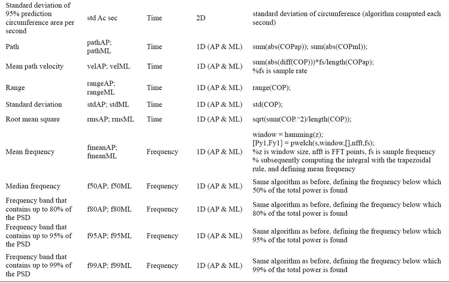
Table 1. Selected traditional parameters and classification.

Figure 2. (a) Exemplary area calculation via 95%- prediction ellipse; (b) Area calculation via the Leibnitz method; (c) Power spectral density of AP direction and parameters (with allowance of [24], modified).
menter. Small variations in those initial values may lead to different results and entrap to error-prone interpretations. Nonetheless, nonlinear tools are believed to be more sensitive and suitable to physiological data [32] and represent complementary information content to traditional methods [33,37,38]. An inspection of literature reveals that this field is continuously rising. On account of the great variety of different nonlinear methods, we abstracted procedures which were chosen in a previously published work to evaluate COP sway data [24].
We applied four different nonlinear tools to 1D AP and 1D ML data, respectively. For our purpose we calculated the sample entropy (SaEn, [39]) of the AP and ML position data and of its velocity time series (increment time series) which gives 4 regularity values and another 2 complexity indices from the multiscale entropy (MSE, [40]). Furthermore we educed one Hurst exponent [5] in AP and ML direction respectively. We combined these measures with a frequency analysis achieved by the Wavelet transform (WT) and computed a total of 2 values for different frequency bands (Figure 3). Overall, we obtained 10 nonlinear measures. A previous work gives a comprehensive overview of the applied nonlinear tools and computations used here [24]. Nonlinear procedures were chosen carefully to obtain best outputs. Table 2 shows the obtained nonlinear parameters.
2.5. General Procedure and Exploratory Factor Analysis
We applied an exploratory factor analysis (EFA) by using SPSS© 17.0 to the preselected linear (traditional) and nonlinear parameters, respectively, as far as both views disclose complementary information. To ensure comparability the parameter values were transformed into zscores. To maintain accurate calculation we conducted the following procedure: 1) Correlation matrix. In this step we proved the suitability of the COP parameters for further analysis. First, we computed Bartlett’s test of sphericity to reject the null hypothesis that the correlation matrix is equal to an identity matrix. Next, the KaiserMeyer-Olkin criterion (KMO) and the anti-image-correlation matrix (AIC) were inspected to test whether partial correlations among variables were small. Variables which showed only a few correlations to other ones had to be excluded. We compared the factor loadings of the remaining parameters to the respective components before and after this exclusion to ensure whether this method anyhow leads to uniform results. The KMO value and the diagonal entries of the AIC (measures of sampling adequacy) should be greater than 0.5 [42]; 2) Extraction. Here, we estimated the factor loadings through an extraction of the factors by means of a PCA. The number of factors was calculated by the Kaiser-Dickmann criterion, meaning, dropping principal components whose eigenvalues are less than one [43]. Furthermore communalities can be computed, which can be seen as a common variance of the item due to the different factor solutions; 3) Rotation method. The factor rotation was achieved by the VARIMAX algorithm to gain maximal variance between factors and therefore to facilitate interpretation.
An apparent emerging problem of the present study is the small sample-size of 16 subjects, which complicates an application and interpretation of factor analysis. The recommendations of methodologists for an adequate sample-size differ and exhibit large ranges. As discussed earlier by [44], sample size has relatively little impact on EFA solutions even with very small cohorts, when communalities of the variables are uniformly high. As reported by [45] item communalities are considered high, if their values are all over 0.8. However, the authors proclaim a caveat to this general assertion that those values are very unlikely to occur in real life data and that more common magnitudes are found in social sciences in a range between 0.4 and 0.7.
Furthermore, using more variables as subjects (subjects-to-variables ratio less than one) is a second prevailing problem for EFA here, leading to a correlation matrix which is not positive definite. On account of this problem we subdivided the parameters into five classes, which are described formerly in the traditional and nonlinear parameters sections and has been similarly explained by others [23]. The traditional parameters are classified into three blocks: 1D time domain and frequency domain parameters (AP), 1D time domain and frequency domain parameters (ML) and 2D parameters comprising 10, 10 and 13 values, respectively. The nonlinear measures form another two blocks in AP and ML direction containing 5 values each. In a first analysis we
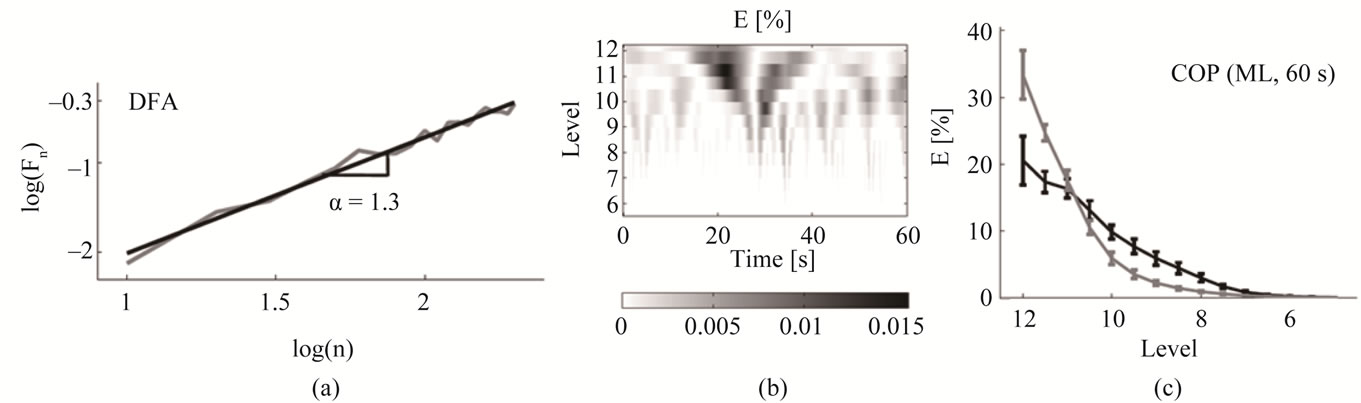
Figure 3. (a) DFA analysis and Hurst exponent; (b) Scalogram of a 12-level Wavelet transform of AP (60 s); (c) Sample mean of energy percentage of the Wavelet transform (with allowance of [24]).
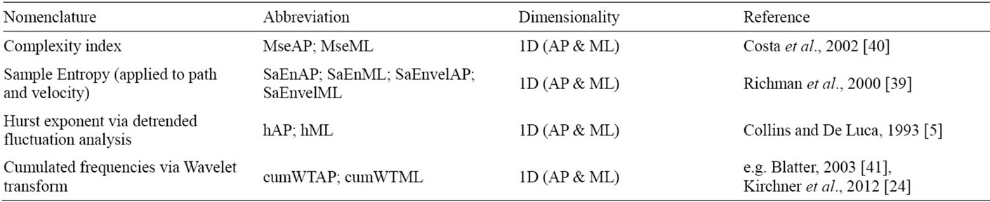
Table 2. Selected nonlinear parameters.
assembled linear and nonlinear parameters in one APand in one ML-group, which unfortunately did not give adequate results regarding sampling adequacy, so that we had to separate linear and nonlinear variables. Within each of the five parameter blocks an exploratory factor analysis was calculated (Figure 1). This was conducted consistently throughout the different measurement times (30 s, 60 s, 300 s), so that a total of 15 EFAs were computed. Rocchi et al. (2004) applied a similar procedure for 1D and 2D parameters [21]. In this article the authors assume that the different groups share most of the information. Here we adopted this keynote by dividing the parameters first into five classes.
3. RESULTS
3.1. Sampling Adequacy
Due to KMO and AIC values we excluded in 4 cases of 15 EFA’s particular parameters to improve the sampling adequacy of the parameter sets. Those were f50AP (30 s, BT, 1D-AP block), Ae and std Ae sec (60 s, BT, 2D block), and SaEnvelAP (300 s, BT, nonlinear AP-block). The exclusion process showed no influence on the remaining parameter loadings. After this procedure the sampling adequacy values matched the requirements (mean KMO = 0.73, KMOmin = 0.68, KMOmax = 0.84). Item communality values were consistently over 0.85 which match the specifications of [44] and [45]. This can be generally explained by high correlations between the stabilometric parameters. As a result, the proband cohort which is smaller than traditionally recommended is likely sufficient for adequate application of EFA [44]. Bartlett’s test of sphericity always rejects the null hypothesis that the correlation matrix is equal to an identity matrix [p < 0.001].
3.2. Traditional Parameters 1D ML
EFA’s from this group (Table 3) show a consistent pattern. All factor loadings regardless of sample duration (30 s, 60 s, 300 s) exhibit two principal components with approximately equal loadings in variance (approximately 40% in the first to 40% in the second component). In a sum the EFA’s explain at about 80% - 90% of variance on average. The principal components are easy to interpret.
The first component refers to parameters from the time domain (pathML, velML, rangeML, stdML and RMSML) and the second component is associated to parameters from the frequency domain (fmeanML, f50ML, f80ML, f95ML and f99ML). Another peculiarity alludes to the individual item loadings in the components. The highest loadings in the frequency parameters have fmeanML, f80ML and f95ML. In the time domain all parameters have similar loadings consistently over 0.9 except of velML. The latter parameter sometimes loads with higher values to the frequency component.
3.3. Traditional Parameters 1D AP
In anterior posterior direction (Table 4) a similar output as in ML direction is interpretable. Two components were extracted at which a distribution of time domain and frequency domain variables is detectable akin to those of the ML direction. An exception is the 60 s trial, in which VelAP creates a third component with 11% of explained variance. The remaining variances are explained by both components equally (approximately 40% in the first component to 40% in the second component) with a total sum of 80% - 90%. Inside the 30 s sample some frequency parameters (fmeanAP, f80AP and f95AP) are also loading negatively to the component which is loaded by the time domain parameters. In the 30 s and 300 s trial VelAP is loading to the frequency component.
3.4. Traditional Parameters 2D
Parameters describing the 2D-COP trace (Table 5) are partitioned into three components normally. Interestingly, there are some general schemes identifiable which are constant over the sampling durations. In general, the first component often comprises five parameters (r, std r, Ah, Ae and Ac, Ac sec and std Ac sec) with some inconsistencies in the 60 s trial (40 to 60% of total variance). This component obviously refers to the global area covering the COP trace. Naturally, the two distance parameters R and std r from normalized COP centre is mathematically strongly related to the area values. A separate component
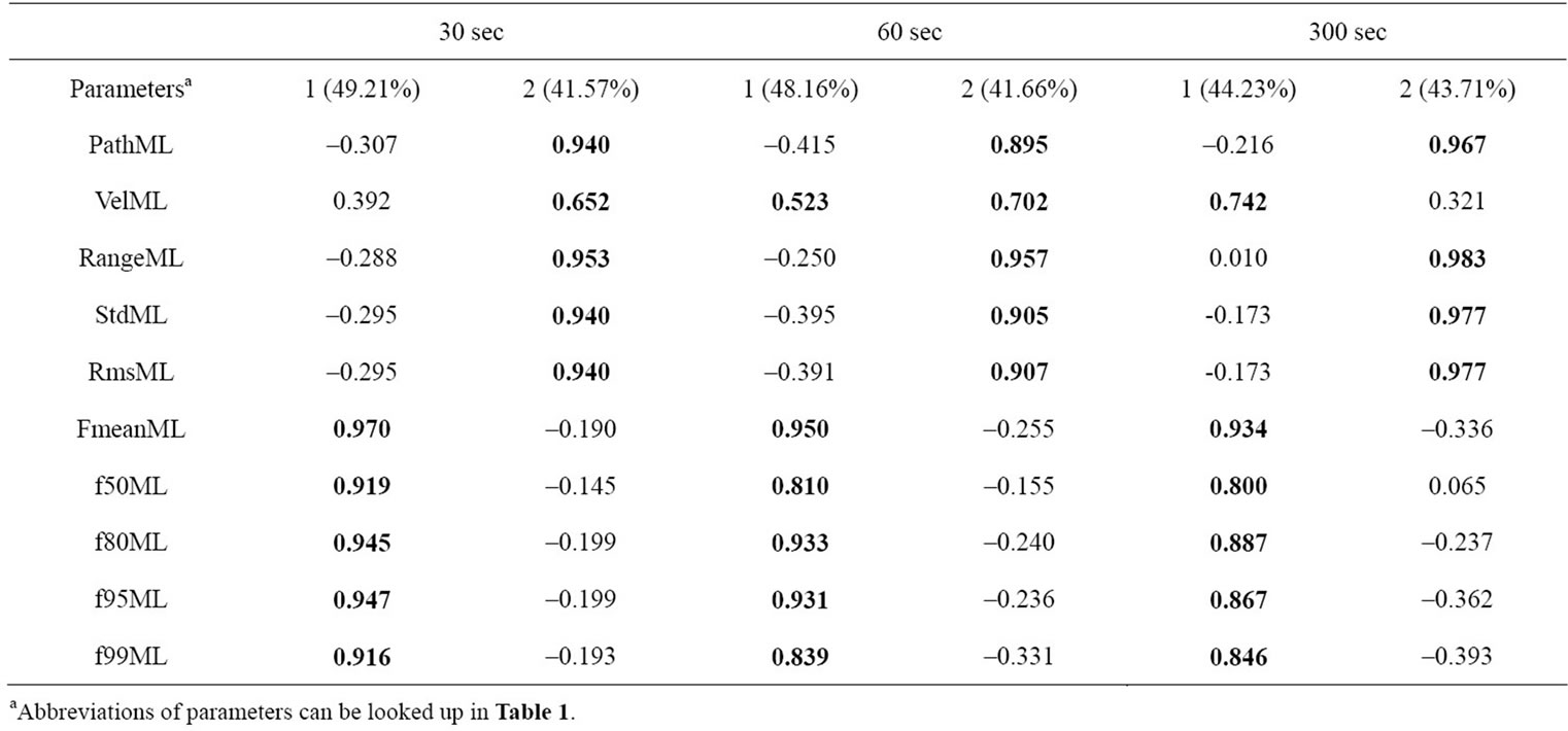
Table 3. Factor loadings for 1-D parameters ML (rotated, >0.5 in bold letters). Components and explained variances.

Table 4. Factor loadings for 1-D parameters AP (rotated, >0.5 in bold letters). Components and explained variances.
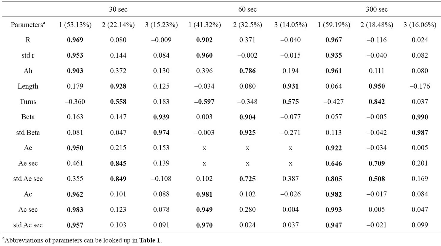
Table 5. Factor loadings for 2-D parameters (rotated, >0.5 in bold letters). Components and explained variances.
is built by Beta and Std Beta (15% to 30% of total variance), which can be interpreted as a global alignment of COP excursion. The third component comprises of Length, Turns and in some cases of Aesec and std Ae sec (14% to 22% of total variance). It may be discerned as 2-dimensional COP path-length characteristics. Moreover, there are specific variable groupings. Remarkably, Ae sec and std Ae sec is not related to Ac sec and std Ac sec. In 30 s and 300 s, mean Ae sec and Std Ae sec both load to a different component as Ae itself, whereas the circular counterparts Ac, Ac sec and std Ac sec are grouped together.
3.5. Nonlinear Parameters ML
In this variable set two components were extracted (Table 6). One component contains the entropy values SaEnML and SaEnvelML, as well as hML (30% to 45% of total variance). The component may be interpreted as a group of values indexing the irregularity of the underlying time series. The second component is generated by the multiscale entropy value and cumWTML. These values account for different time scales (different time scales in the entropy algorithm, and different frequency bands via wavelet transform). Hence, this component can be seen as a global nonlinear interpreter of the underlying time series in medial lateral direction. Despite this interpretation of the components slight differences in individual loadings are preexisting. Referring to this hML in the 30 s set-up is loading to both components, and the same fact is given by SaEnML in 60 s and 300 s.
3.6. Nonlinear Parameters AP
In this nonlinear group (Table 7) two components are extracted. The factor loadings here are insofar comparable to ML as MseAP is related to cumWTAP. SaEnAP is attached to this component (40% to 60% of total variance). The second component is roughly based on the entropy value SaEnvelAP and the Hurst coefficient hAP. However, AP case does not reveal an equal structure compared to the ML parameter set. The interpretation of the two components seems to be different. We will account for the 300 s trial to have better discriminative power in factor configuration [7,24]. Therefore, the components are based on the same variables as in the ML set (MseAP and cumWTAP in the first component, the entropy values in the second one).
4. DISCUSSION
4.1. Effect of Sampling Duration on COP Parametrization
Standing as still as possible on a plane and stable surface is a prime indicator for postural control and approves investigation of sway dynamics in research and in a clinical context. However, lack of standardization in static posturography experiments complicates the comparison of results between different studies. As a consequence this has led to contradictory outcomes which hamper
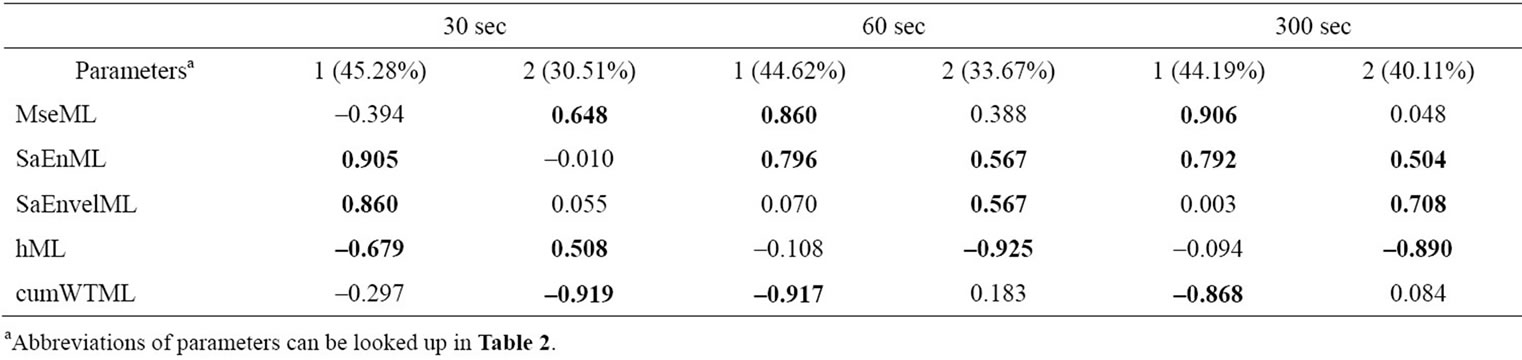
Table 6. Factor loadings for nonlinear parameters ML (rotated, >0.5 in bold letters). Components and explained variances.

Table 7. Factor loadings for nonlinear parameters AP (rotated, >0.5 in bold letters). Components and explained variances.
easy utility in clinical practice [6,29]. Longer sampling durations contain different type of information compared to shorter ones and therefore, this could emerge as a critical factor for obtaining reliable COP data [27]. This is partly underlined by the present study as sampling duration effects concerning particular parameters (VelML, VelAP, Aesec, std Ae sec, SaEnML, hML, and SaEnAP) are revealed. VelML and VelAP display relations to frequency parameters when the sampling duration is 300 s, which may be an effect due to better resolution in the low frequency range. Ae sec and std Ae sec seem to come along with area values as well as pathlength parameters in longer durations. The underlying computation every second implies that the major axis of the ellipse points to the COP displacement direction which carries more weight within longer durations. SaEnML and hML are loading consistently in 60 and 300 s and SaEnAP changes its affinity to one component with 300 s. One can speculate if longer durations serve as better estimates for these values. With respect to traditional parameters, longer sampling durations apparently enables higher reliability values within the COP data set [7,27]. In a recent paper Kirchner et al. (2012) have shown that longer recording times (≥60 s) seems to have more discriminative power for nonlinear measures than shorter ones [24]. Regarding frequency components of time series longer sample durations come along with a decomposition of lower frequency contents in the data. Since COP excursions compose of 95% of the frequency power beneath 1 Hz, longer durations account for better resolution [24,28]. The longer the sampling durations the less transient events have an impact on time series and the more extreme values could be detected as an appendix of the physiological process. A second prevailing problem in standardization in COP studies refers to the choice of posturographic parameters. It is well-established, that a set of parameters is needed to declare most of the variance in COP data [21,23,30,34]. However, an influence of recording times on the choice of parameters within parametrization sets is left unknown. The present study aims the question whether sampling duration affects the choice of posturographic parameters, and hence delivers a straightforward framework for COP standardization. Considering the pattern of the five parameter groups inside the different measurement times (30 s, 60 s, 300 s) a minor effect on parameter setting has been revealed. Despite the aforementioned dependencies on sampling durations for some parameters, all in all, factor loadings show consistent pattern throughout all groupings. Hence, a similar set of parameters may be used in spite of different sampling durations. We would like to point out that this result does not favor short sampling durations, but that even within shorter recording durations, explanation of COP data could be achieved through an equal set of parameters as it is proposed in longer measurement times. Short sampling durations may be useful for subjects who are unable to stand longer than 30 s. In this case more repetitions in quiet standing task are required to gain appropriate reliability of results [27]. Furthermore, a set of nonlinear parameters has been included into a comprehensive analysis involving entropy values, DFA and wavelet transform.
4.2. Classification of Parameters
A prime aspect of standardization involves the usage of a comprehensive set of descriptive posturographic parameters [6]. There exists a great variety of COP descriptors and diverse recommendations on the usage of these parameters have been published. Rocchi et al. (2004) decomposed the COP data in a 1-dimensional and a 2-dimensional group of variables and derived four and six parameters respectively via principal component analysis [21]. Designed according to this, the parameters are subdivided into five groups which presumably share most of the information: 1-dimensional AP and ML, 2-dimensional, and nonlinear AP and ML. A feature of the present study is a separate variable block containing exclusively nonlinear values (sample entropy measures, complexity index and a value derived from the wavelet transform), for which calculation is more sophisticated. Compared to traditional variables, these measures are believed to be more sensitive to diverse aspects of signal processing and are applied in order to understand physiological variability [32,33]. The several groups possess different components for which in each case one representative parameter has to be chosen. This study presents a parametrization framework and we make some proposals to obtain particular posturographic parameters based on the predefined groups. One can speculate whether different configurations would reveal different component pattern. For instance, assembling linear and nonlinear parameters in one group may give an insight into the interactions of both variable characteristics [46]. However, this approach had to be abandoned due to bad sampling adequacy results. Inside the 1-dimensional group a time domain and a frequency domain component is disclosed. Time domain parameters comprise mostly variables describing the magnitude of the time series. In this regard, posturographic measures that refer to just a few representative points among the entire time series should be avoided [27]. Here, outliers are responsible for great variances and hence low reliability. Other measures that explain the magnitude of the 1-dimensional time series had to be preferred, like std or rms (both variables are highly correlated). Indeed, latter variables are more robust, even though, they present vulnerable values confronting outliers as well. Within the frequency domain we recommend F80, as far as [47] demonstrated F80 having best statistical performance in opposition to F70, F85, F90 or F95. The 2-dimensional parameters display three components: the global area which covers the COP trace, the global alignment of the COP path, and the COP path-length characteristics. COP area may be highlighted using Ah, as this measure is the best estimate, followed by Ae and Ac. The global alignment should be determined with the AP angle deviance beta, which has been earlier recommended by [21]. Concerning path-length characteristics, some authors underline the significance of COP velocity as the most reliable indicator of global COP migration [48,49]. As we mention before, this variable correlates perfectly with the COP length. The nonlinear group is divided into two components. The choice of a regularity index is more difficult to arrange as this is strongly dependant on the underlying algorithm. We recommend sample entropy SaEn introduced by [39] as it shows better relative consistency and is less sensitive to the lengths of data time series compared to other algorithms [24]. The nonlinear value encompassing different time scales is to our opinion achieved through cumWT values. Wavelet transform is able to decompose a signal into different frequency bands within different time scales which avoids the problem that comes along with Fast Fourier Transform-frequency and time resolution [24].
5. CONCLUSION
We demonstrate that COP evaluation irrespective of sampling duration necessitates a set of diverse parameters to gain more variance of the data. Parameter sets are—despite of a few exceptions—uniformly invariant towards sampling durations and display a consistent factor loading pattern. 11 parameter groups are suggested for COP evaluation. A comprehensive analysis of posturography should imply descriptive measures regarding the 2-dimensional COP trace and the decomposed 1-dimensional AP and ML time series to gain maximal explanation of variance in COP data: three global (2-dimensional) parameters: 1) area; 2) alignment; 3) path-length characteristics, eight 1-dimensional parameters; 4) time domain AP; 5) time domain ML; 6) frequency domain AP; 7) frequency domain ML; 8) irregularity parameter AP; 9) irregularity parameter ML; 10) nonlinear multi-timescale parameter AP; and 11) nonlinear multi-timescale parameter ML. This study suggests a framework for standardization of parameter sets within these subgroups. Furthermore this study constitutes a critical position on studies that has just included a few parameters for COP description.
6. ACKNOWLEDGEMENTS
This research was supported by the LOEWE focus “PreBionics”.
![]()
![]()
REFERENCES
- Winter, D. (2009) Biomechanics and motor control of human movement. 3rd Edition, John Wiley & Sons, Hoboken.
- Latash, M. (2008) Neurophysiological basis of movement. 2nd Edition, Human Kinetics, Champaign.
- Chagdes, J., Rietdyk, S., Haddad, J., Zelaznik, H., Raman, A., Rhea, C. and Silver, T. (2009) Multiple timescales in postural dynamics associated with vision and a secondary task are revealed by wavelet analysis. Experimental Brain Research, 197, 297-310. doi:10.1007/s00221-009-1915-1
- Deliagina, T.G., Orlovsky, G.N., Zelenin, P.V. and Beloozerova I.N. (2006) Neural bases of postural control. Physiology, 21, 216-225. doi:10.1152/physiol.00001.2006
- Collins, J. and De Luca, C. (1993) Open-loop and closedloop control of posture: A random-walk analysis of center-of-pressure trajectories. Experimental Brain Research, 95, 308-318. doi:10.1007/BF00229788
- Visser, J.E., Carpenter, M.G., Van der Kooij, H. and Bloem, B.R. (2008) The clinical utility of posturography. Clinical Neurophysiology, 119, 2424-2436. doi:10.1016/j.clinph.2008.07.220
- Van der Kooij, H., Campbell, A.D. and Carpenter, M.G. (2011) Sampling duration effects on centre of pressure descriptive measures. Gait & Posture, 34, 19-24. doi:10.1016/j.gaitpost.2011.02.025
- Vuillerme, N. and Nafati, G. (2007) How attentional focus on body sway affects postural control during quiet standing. Psychological Research, 71, 192-200. doi:10.1007/s00426-005-0018-2
- Fraizer, E. and Mitra, S. (2008) Methodological and interpretive issues in posture-cognition dual-tasking in upright stance. Gait Posture, 27, 271-279. doi:10.1016/j.gaitpost.2007.04.002
- Wulf, G., Mercer, J., McNevin, N. and Guadagnoli, M.A. (2004) Reciprocal influences of attentional focus on postural and suprapostural task performance. Journal of Motor Behavior, 36, 189-199. doi:10.3200/JMBR.36.2.189-199
- Laughton, C.A., Slavin, M., Katdare, K., Nolan, L., Bean, J.F., Kerrigan, D.C., Phillips, E., Lipsitz, L.A. and Collins, J.J. (2003) Aging, muscle activity, and balance control: Physiologic changes associated with balance impairment. Gait & Posture, 18, 101-108. doi:10.1016/S0966-6362(02)00200-X
- Le Clair, K. and Riach, C. (1993) Postural stability measures: What to measure and for how long. Clinical Biomechanics, 11, 176-178. doi:10.1016/0268-0033(95)00027-5
- Duarte, M. and Sternard, D. (2008) Complexity of human postural control in young and older adults during prolonged standing. Experimental Brain Research, 191, 265- 276. doi:10.1007/s00221-008-1521-7
- Freitas, S.M.S.F., Wieczorek, S.A., Marchetti, P.H. and Duarte, M. (2005) Age-related changes in human postural control of prolonged standing. Gait & Posture, 22, 322- 330. doi: 10.1016/j.gaitpost.2004.11.001
- Duarte, M., Harvey, W. and Zatsiorsky, V.M. (2000) Stabilographic analysis of unconstrained standing. Ergonomics, 43, 1824-1839. doi:10.1080/00140130050174491
- Carpenter, M.G., Frank, J.S., Winter, D.A. and Peysar, G.W. (2001) Sampling duration effects on centre of pressure summary measures. Gait and Posture, 13, 35-40. doi:10.1016/S0966-6362(00)00093-X
- Duarte, M., Freitas, S.M.S.F. and Zatsiorsky, V. (2011) Control of equilibrium in humans—Sway over sway. In: Latash, M. and Danion, F., Eds., Motor Control, Oxford University Press, Oxford, 219-242.
- Duarte, M. and Zatsiorsky, V.M. (1999) Patterns of center of pressure migration during prolonged unconstrained standing. Motor Control, 3, 12-27.
- Carrol, J.P. and Freedman, W. (1993) Nonstationary properties of postural sway. Journal of Biomechanics, 26, 409-416. doi:10.1016/0021-9290(93)90004-X
- Riley, M.A., Balasubramaniam, R. and Turvey, M.T. (1999) Recurrence quantification analysis of postural fluctuations. Gait and Posture, 9, 65-78. doi:10.1016/S0966-6362(98)00044-7
- Rocchi, L., Chiari, L. and Capello, A. (2004) Feature selection of stabilometricparameters based on principal component analysis. Medical & Biological Engineering & Computing, 42, 71-79. doi:10.1007/BF02351013
- Pavol, M.J. (2005) Detecting and understanding differences in postural sway. Focus on “a new interpretation of spontaneous sway measures based on a simple model of human postural control”. Journal of Neurophysiology, 93, 20-21. doi:10.1152/jn.00864.2004
- Kitibayashi, T., Demura, S. and Noda, M. (2003) Examination of the factor structure of center of foot pressure movement and cross-validity. Journal of Physiological Anthropology and Applied Human Science, 22, 265-272. doi:10.2114/jpa.22.265
- Kirchner, M., Schubert, P., Schmidtbleicher, D. and Haas, C.T. (2012) Evaluation of the temporal structure of postural sway fluctuations based on a comprehensive set of analysis tools. Physica A, 391, 4692-4703. doi:10.1016/j.physa.2012.05.034
- Bolbecker, A.R., Hong, S.L., Kent, J.S., Klaunig, M.J., O’Donnell, B.F. and Hetrick, W.P. (2011). Postural control in bipolar disorder: Increased sway area and decreased dynamical complexity. Plos ONE, 6, e19824 doi:10.1371/journal.pone.0019824
- Prado, J., Stoffregen, T. and Duarte, M. (2007) Postural sway during dual tasks in young and elderly adults. Gerontology, 53, 274-281. doi:10.1159/000102938
- Ruhe, A., Fejer, R. and Walker, B. (2010) The test-retest reliability of centre of pressure measures in bipedal static task conditions—A systematic review of the literature. Gait & Posture, 32, 436-445. doi:10.1016/j.gaitpost.2010.09.012
- Maurer, C. and Peterka, R. (2005) A new interpretation of spontaneous sway measures based on a simple model of human postural control. Journal of Neurophysiology, 93, 189-200. doi:10.1152/jn.00221.2004
- Duarte, M. and Freitas, S. (2010) Revision of posturography based on force plate for balance evaluation. Revista Brasileira de Fisioterapia, 14, 183-192. doi:10.1590/S1413-35552010000300003
- Prieto, T., Myklebust, J., Hoffmann, R., Lovett, E. and Myklebust, B. (1996) Measures of postural steadiness: Differences between healthy young and elderly adults. IEEE Transactions on Biomedical Engineering, 43, 956- 966. doi:10.1109/10.532130
- Raymakers, J.A., Samson, M.M. and Verhaar, H.J.J. (2005) The assessment of body sway and the choice of the stability parameter(s). Gait & Posture, 21, 48-58. doi:10.1016/j.gaitpost.2003.11.006
- Stergiou, N. and Decker, L.M. (2011) Human movement variability, nonlinear dynamics, and pathology: Is there a connection? Human Movement Science, 30, 869-888. doi:10.1016/j.humov.2011.06.002
- Harbourne, R. and Stergiou, N. (2009) Movement variability and the use of nonlinear tools: Principles to guide physical therapist practice. Physical Therapy, 89, 267-283. doi:10.2522/ptj.20080130
- Demura, S., Kitibayashi, T. and Noda, M. (2006) Selection of useful parameters to evaluate center-of-foot pressure movement. Perceptual and Motor Skills, 103, 959- 973. doi:10.2466/PMS.103.7.959-973
- Rocchi, M.B.L., Sisti, D., Ditroilo, M., Calavalle, A. and Panebianco, R. (2005) The misuse of the confidence ellipse in evaluating statokinesigram. International Journal of Sports Science, 12, 169-171.
- Donker, S.F., Roerdink, M., Greven, A.J. and Beek, P.J. (2007) Regularity of center-of-pressure trajectories depends on the amount of attention invested in postural control. Experimental Brain Research, 181, 1-11. doi:10.1007/s00221-007-0905-4
- Stergiou, N., Harbourne, R. and Cavanaugh, J. (2006) Optimal movement variability: A new theoretical perspective for neurologic physical therapy. Journal of Neurologic Physical Therapy, 30, 120-130.
- Cavanaugh, J.T., Mercer, V.S. and Stergiou, N. (2007) Approximate entropy detects the effect of a secondary cognitive task on postural control in healthy young adults: A methodological report. Journal of NeuroEngineering and Rehabilitation, 4, 1-7. doi:10.1186/1743-0003-4-42
- Richman, J. and Moorman, J. (2000) Physiological timeseries analysis using approximate entropy and sample entropy. American Journal of Physiology—Heart and Circulatory Physiology, 278, H2039-H2049.
- Costa, M., Goldberger, A. and Peng, C. (2002) Multiscale entropy analysis of complex phyiologic time series. Physical Review Letters, 89, 068102. doi:10.1103/PhysRevLett.89.068102
- Blatter, C. (2003) Wavelets—An introduction (German title: Wavelets—Eine Einführung). 2nd Edition, Vieweg, Brunswick.
- Kaiser, H.F. (1974) An index of factorial simplicity. Psychometrica, 39, 31-36. doi:10.1007/BF02291575
- Kaiser, H.F. (1960) The application of electronic computers to factor analysis. Educational and Psychological Measurement, 20, 141-151. doi:10.1177/001316446002000116
- MacCallum, R.C., Widaman, K.F., Zhang, S. and Hong, S. (1999) Sample size in factor analysis. Psychological Methods, 4, 84-99. doi:10.1037/1082-989X.4.1.84
- Costello, A.B. and Osborne, J.W. (2005) Best practices in exploratory factor analysis: Four recommendations for getting the most from your analysis. Practical Assessment, Research & Evaluation, 10, 1-9.
- Harbourne, R.T., Deffeyes, J.E., Kyvelidou, A. and Stergiou, N. (2009) Complexity of postural control in infants: linear and nonlinear features revealed by principal component analysis. Nonlinear Dynamics, Psychology, and Life Sciences, 13, 123-144.
- Baratto, L., Morasso, P.G., Re, C. and Spada, G. (2002) A new look at posturographic analysis in the clinical context: Sway-density vs. other parameterization techniques. Motor Control, 6, 246-270.
- Cornilleau-Pérès, V., Shabana, N., Droulez, J., Goh, J.C.H., Lee, G.S.M. and Chew, P.T.K. (2005) Measurement of the visual contribution to postural steadiness from the COP movement: Methodology and reliability. Gait & Posture, 22, 96-106. doi:10.1016/j.gaitpost.2004.07.009
- Lafond, D., Corriveau, H., Hébert, R. and Prince, F. (2004) Intrasession reliability of center of pressure measures of postural steadiness in healthy elderly people. Archives of Physical Medicine and Rehabilitation, 85, 896-901. doi:10.1016/j.apmr.2003.08.089
NOTES
*Corresponding author.