Intelligent Information Management
Vol.5 No.4(2013), Article ID:34702,9 pages DOI:10.4236/iim.2013.54012
Estimation Based on Progressive First-Failure Censored Sampling with Binomial Removals*
1Faculty of Science, Islamic University, Madinah, Saudi Arabia
2Mathematics Department, Sohag University, Sohag, Egypt
3Mathematics Department, Faculty of Science, Al-Azhar University, Nasr-City, Cairo, Egypt
Email: Rashadmath@yahoo.com
Copyright © 2013 Ahmed A. Soliman et al. This is an open access article distributed under the Creative Commons Attribution License, which permits unrestricted use, distribution, and reproduction in any medium, provided the original work is properly cited.
Received April 27, 2013; revised May 28, 2013; accepted June 15, 2013
Keywords: Burr-X Distribution; Progressive First-Failure Censored; Bayesian and Non-Bayesian Estimations; Loss Function; Bootstrap; Random Removals
ABSTRACT
In this paper, the inference for the Burr-X model under progressively first-failure censoring scheme is discussed. Based on this new censoring were the number of units removed at each failure time has a discrete binomial distribution. The maximum likelihood, Bootstrap and Bayes estimates for the Burr-X distribution are obtained. The Bayes estimators are obtained using both the symmetric and asymmetric loss functions. Approximate confidence interval and highest posterior density interval (HPDI) are discussed. A numerical example is provided to illustrate the proposed estimation methods developed here. The maximum likelihood and the different Bayes estimates are compared via a Monte Carlo simulation study.
1. Introduction
Censoring is common in life-distribution work because of time limits and other restrictions on data collection. Censoring occurs when exact lifetimes are known only for a portion of the individuals or units under study, while for the remainder of the lifetimes information on them is partial. However, when the lifetimes of products are very high, the experimental time of a type II censoring life test can be still too long. A generalization of type II censoring is progressive type II censoring, which is useful when the loss of live test units at points other than the termination point is unavoidable. Johnson [1] described a life test in which the experimenter might decide how to group the test units into several sets, each as an assembly of test units, and then run all the test units simultaneously until occurrence of the first failure in each group. Such a censoring scheme is called first-failure censoring. Wu and Kuş [2] obtained maximum likelihood estimates, exact confidence intervals and exact confidence regions for the parameters of Weibull distribution under the progressive first-failure censored sampling. Note that a firstfailure censoring scheme is terminated when the first failure in each set is observed. If an experimenter desires to remove some sets of test units before observing the first failures in these sets this life test plan is called a progressive first-failure censoring scheme which recently was introduced by Wu and Kuş [2]. Recently, the estimation of Parameters from different lifetime distribution based on progressive type II censored samples is studied by several authors including Gupta et al. [3], Childs and Balakrishnan [4], Siu keung tse et al. [5], Mosa and Jaheen [6], Ng et al. [7], Wu and Chang [8], Balakrishnan et al. [9], Wu [10], Soliman [11], and Sarhan and Abuammoh [12]. But in some reliability experiments, the number of patients dropped out the experiment cannot be pre-fixed and it is random. In such situations, the progressive censoring schemes with random removals are needed. Therefore, the purpose of this paper is to develop a Bayes estimation (symmetric and asymmetric loss functions) for the parameters of Burr-X distribution under the progressive first-failure censoring plan with random removals and construct the bootstrap confidence interval for the parameters.
If  follows a Burr-X distribution, then the probability density function (pdf) and cumulative distribution function (cdf) of
  are given respectively by
 (1)
(1)
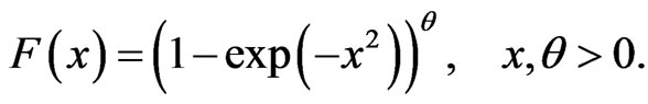 (2)
(2)
The rest of this paper is organized as follows. In Section 2, we describe the formulation of a progressive firstfailure censoring scheme as described by Wu and Kuş [2]. The point estimation of the parameters of Burr-X distribution and binomial distribution based on the progressive first-failure censoring scheme is investigated in Section 3. In Section 4, we discuss the approximate interval estimation and highest posterior density interval (HPDI) for the Burr-X distribution under the progressive first-failure censored sampling plan. A numerical examples are presented in Section 5, for illustration. In Section 6 we provide some simulation results in order to give an assessment of the performance of the estimation method.
2. A Progressive First-Failure Censoring Scheme
In this section, first-failure censoring is combined with progressive censoring as in Wu and Kuş [2]. Suppose that n independent groups with  items within each group are put in a life test,
  groups and the group in which the first failure is observed are randomly removed from the test as soon as the first failure (say
 ) has occurred,
  groups and the group in which the second failure is observed are randomly removed from the test as soon as the second failure (say
 ) has occurred, and finally
  groups and the group in which the
  failure is observed are randomly removed from the test as soon as the
  failure (say
  ) has occurred. The
  are called progressively first-failure-censored order statistics with the progressive censoring scheme
 . It is clear that
  . If the failure times of the
  items originally in the test are from a continuous population with distribution function
  and probability density function
 , the joint probability density function for
 is given by
 (3)
(3)
 (4)
(4)
where
 (5)
(5)
There are four special cases:
The first one if , Equation
  reduces to the joint probability density function of first-failurecensored order statistics. The second case if
 , Equation (3) becomes the joint probability density function of the progressively type II censored statistics. The third case if
  and
and , then
  which corresponds to the complete sample. The last one if
  and
and , then type II censored order statistics are obtained.
Also it can be seen that  can be viewed as a progressively type II censored sample from a population with distribution function
  . For this reason, results for the progressively type II censored order statistics can be extended to progressively first-failure-censored order statistics easily.
Obviously, although more items are used (only  of
of  items are failures) in the progressive first-failure censoring plan than in others, it has advantages in terms of reducing test cost and test time.
3. Point Estimation
In many cases, there will be an obvious or natural candidate for a point estimator of a particular parameter. For example, the sample mean is a natural candidate for a point estimator of the population mean. In this section, we estimate  and
and , by considering maximum likelihood, bootstrap and Bayes estimates. In Bayesian technique, we consider both symmetric (Squares Error, SE) loss function and asymmetric (Linear Exponential, LINEX and General Entropy, GE) loss functions.
3.1. Maximum Likelihood Estimation (MLE)
Let ,
, , be the progressively first-failure censored order statistics from a Burr-X distribution, with censoring scheme
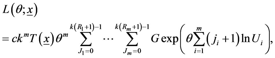
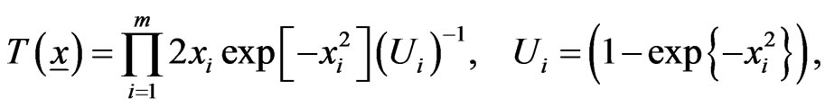
  from (3), the likelihood function is given by
 (6)
(6)
where
 (7)
(7)
 (8)
(8)
where  is defined in (5) and
  is used instead of
 . Now, suppose that any group
  being removed from the life test is independent of the others but with the same probability
 . Then, the number of groups removed at each failure time follows a binomial distribution with parameters
  and
and  where
where  is predetermined before the testing. Therefore
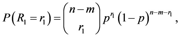 (9)
(9)
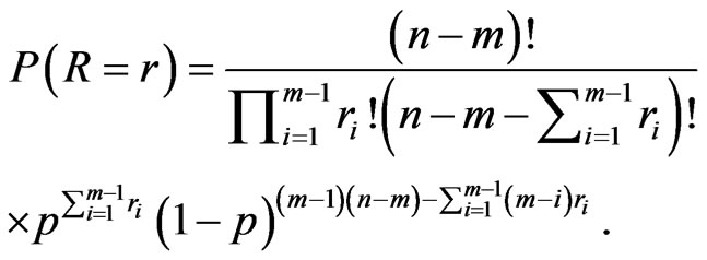
and for 
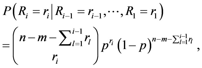 (10)
(10)
where 

 (11)
(11)
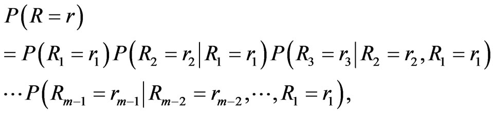
hence
 (12)
(12)
Suppose further that  is independent of
 . Then the likelihood function takes the following form
 (13)
(13)
 (14)
(14)
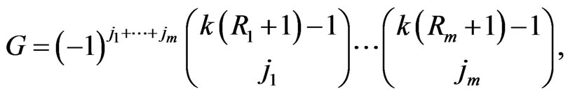
Using (6), (12) and (13) we can write the likelihood function as
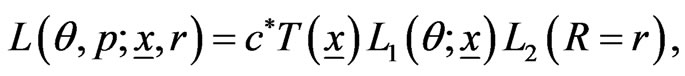 (15)
(15)
where  and
and
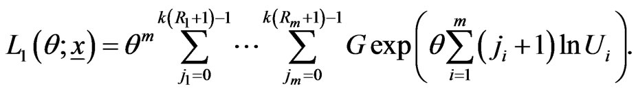 (16)
(16)
and
 (17)
(17)
It is obvious that  in Equation (16) does not involve
 . Thus the maximum likelihood estimate (MLE) of
  can be derived by maximizing Equation (16) directly. On the other hand,
  in Equation (17) does not depend on the parameter
  then the MLE of
  can be obtained directly by maximizing Equation (17). In particular, after taking the logarithms of
  and
and , the MLE’s of
  and
and  can be found by solving the following equations
 (18)
(18)
 (19)
(19)
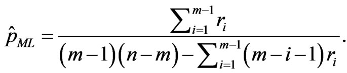
Thus we find
 (20)
(20)
and 
 (21)
(21)
3.2. Bootstrap Confidence Intervals
In this subsection, we use the parametric bootstrap percentile method suggested by Efron [13] to construct confidence intervals for the parameters. The following steps are followed to obtain a progressive first-failure censoring bootstrap sample from Burr-X distribution with parameter  and binomial distribution with parameter
  based on simulated progressively first-failure censored data with random removals set.
• From the original data  and
and  compute the ML estimates of the parameters
  and
and  by Equations (20) and (21).
• Use  and
and  to generate a bootstrap sample
  and
and  with the same values of
  using algorithm presented in Balakrishnan and Sandhu [14] with distribution func• tion
  see Wu and Kuş [2].
• As in Step 1, based on  compute the bootstrap sample estimates of
  and
and  say
say  and
and 
• Repeat steps 2-3  times representing
  bootstrap MLE’s of
  based on
  different bootstrap samples.
• Arrange all  and
and  in an ascending order to obtain the bootstrap sample
 (where
 ).
).
Let  be the cumulative distribution function of
  Define
  for given z. The approximate bootstrap
  confidence interval of
  is given by
 (22)
(22)
3.3. Bayes Estimation
The Bayesian inference procedures have been developed under the usual SE loss function (quadratic loss), which is symmetrical, and associates equal importance to the losses due to overestimation and underestimation of equal magnitude. However, such a restriction may be impractical. For example, in the estimation of reliability and failure rate functions, an overestimation is usually much more serious than an underestimation; in this case the use of asymmetrical loss function might be inappropriate, as has been recognized by Basu and Ebrahimi [15], and Canfield [16].
A useful asymmetric loss known as the LINEX loss function, was introduced by Zimmer et al. [17], and was widely used in several papers by Balasooriya and Balakrishnan [18], Soliman [19] and Soliman [20]. This function rises approximately exponentially on one side of zero, and approximately linearly on the other side. Under the assumption that the minimal loss occurs at , the LINEX loss function for
  can be expressed as
 (23)
(23)
where  is an estimate of
 .
.
The sign, and magnitude of  represent the direction, and degree of symmetry. (
 means overestimation is more serious than underestimation, and
  means the opposite). For
  closed to zero, the LINEX loss function is approximately the Squared Error (SE) loss, and therefore almost symmetric The posterior-expectation of the LINEX loss function of (23) is
 (24)
(24)
where  is equivalent to the posterior-expectation with respect to the posterior
 . The Bayes estimator
  of
of  under the LINEX loss function is the value
 , which minimizes (24)
 (25)
(25)
provided that  exists, and is finite.
Another useful asymmetric loss function is General Entropy (GE) loss
 (26)
(26)
whose minimum occurs at . This loss function is a generalization of the Entropy-loss used in several papers where
  by Dey et al. [21], Dey and Liu [22]. When
 , a positive error
  causes more serious consequences than a negative error. The Bayes estimate
  of
of  under GE loss (26) is
 (27)
(27)
provided that  exists, and is finite.
Now, we assume that the parameters  and
and  behave as independent random variables, and we use gamma prior distribution with known parameters
  for
for  The prior pdf of
  takes the form
 (28)
(28)
while  has Beta prior distribution with known parameters
  That is
 (29)
(29)
Therefore the posterior (pdf) of  is
is
 (30)
(30)
where  the likelihood function and
  the prior density function. Applying (16) and (28), the marginal posterior (pdf) of
  given by
 (31)
(31)
where
 (32)
(32)
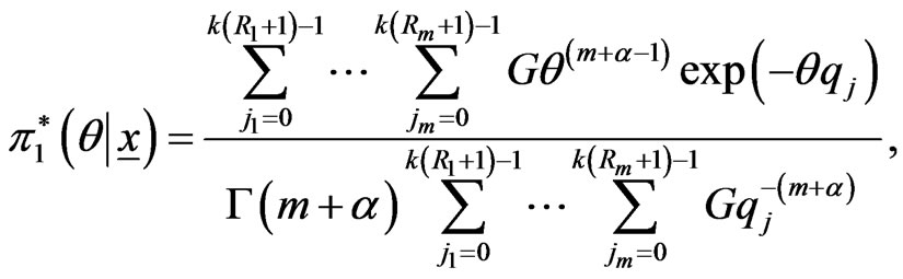
We notes that the posterior distribution of  is Gamma with parameters
  and
and  Similarly, the posterior (pdf) of
  is
is
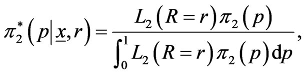 (33)
(33)
where  the likelihood function and
  the prior density function.
Applying (17) and (29), the marginal posterior pdf of  given by
 (34)
(34)
where
 (35)
(35)
We notes that the posterior distribution of  is Beta with parameters
  and
and .
.
3.3.1. Symmetric Bayes Estimation
SE loss function: Under SE loss function, the estimator of a parameter (or given function of the parameters) is its posterior mean. Thus, Bayes estimators of the parameters are obtained by using the posterior densities (31) and (34). The Bayes estimators  and
and  of the parameters
  and
and  are
are
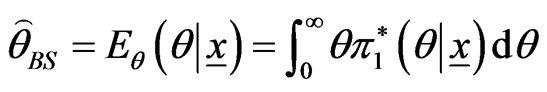 (36)
(36)
from (31) resulting in
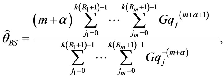 (37)
(37)
where  and
and  are defined in (8) and (32). Similarly,
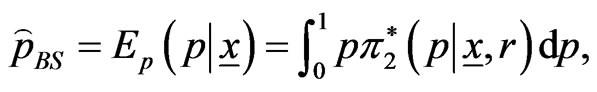 (38)
(38)
from (34) resulting in
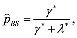 (39)
(39)
where  and
and  are defined in (35).
3.3.2. Asymmetric Bayes Estimation
LINEX loss function: If in (25),  , then the Bayes estimator
  , of the parameter
  relative to LINEX loss function is
 (40)
(40)
and from (31), we get
 (41)
(41)
Similarly, if in (25),  , then the Bayes estimator
 , of the parameter
  relative to LINEX loss function is
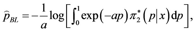 (42)
(42)
and from (34), we obtain
 (43)
(43)
One can use a numerical integration technique to get the integration in (43).
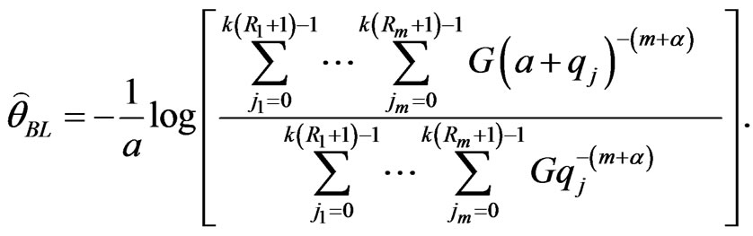
General Entropy loss function: Let , in (27), then the Bayes estimate
 , of parameter
  relative to the General Entropy loss function is
 (44)
(44)
and from (31), we obtain
 (45)
(45)
Put  in (27), then the Bayes estimator
  of the parameter
  relative to General Entropy loss function is
 (46)
(46)
from (34), resulting in
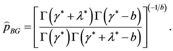 (47)
(47)
4. Interval Estimation
4.1. Approximate Interval Estimation
The asymptotic variances and covariances of the MLE for parameters  and
and  are given by elements of the inverse of the Fisher information matrix
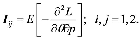 (48)
(48)
Unfortunately, the exact mathematical expressions for the above expectations are very difficult to obtain. Therefore, we give the approximate (observed) asymptotic varaince-covariance matrix for the MLE, which is obtained by dropping the expectation operator E
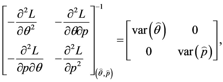 (49)
(49)
with
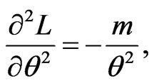 (50)
(50)
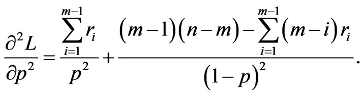 (51)
(51)
The asymptotic normality of the MLE can be used to compute the approximate confidence intervals for parameters  and
and . Therefore,
  confidence intervals for parameters
  and
and  become
 (52)
(52)
where  is the percentile of the standard normal distribution with right-tail probability
 .
.
4.2. Highest Posterior Density Interval (HPDI)
In general, the Bayesian interval estimation is much more direct than frquentest classical method. Now, having obtained the posterior distribution  we ask, “How likely is it that the parameter
  lies within the specified interval
 ?” Bayesian call this interval based on the posterior distribution a “credible interval”. The interval
  is said to be a
  credible interval for
  if
if
 (53)
(53)
For the shortest credible interval, we have to minimize the interval  subject to the condition (53) which requires
 (54)
(54)
As interval  which simultaneously satisfies (53) and (54) is called the “shortest”
  credible interval. A highest posterior density interval (HPDI) is such that the posterior density for every point inside the interval is greater than that for every point outside of it. For a unimodal, but not necessarily symmetrical posterior density, the shortest credible and the HPD intervals are identical. We now proceed to obtain the
 HPD intervals for the parameters
  and
and  Consider the posterior distribution of
  in (31). The
  HPDI
HPDI  for the parameter
  is given by the simultaneous solution of the equations
 (55)
(55)
Similarly, using the posterior pdf of  in (34), the
  HPDI
HPDI  for the parameter
  is given by the simultaneous solution of the equations
 (56)
(56)
To obtain the HPDI from (55) and (56), one may employ any mathematical package such as Mathematica, to get the intervals.
5. Numerical Example
Example 1: (simulated data) To illustrate the use of the estimation methods proposed in this paper. A set of data consisting of 75 observations were generated from a Burr-X distribution with parameter , and randomly grouped into 15 sets. The generated data are listed below:

Now, we consider the following cases:
Case I: Progressive first-failure censored data with binomial removals.
Algorithm 1.
1) Specify the value of 
2) Specify the value of 
3) Generate the value of the parameters  and
and  using the prior densities (28) and (29), for some given values of the prior parameters
  and
and 
4) Generate a random number  from
from 
5) Generate a random numbers  from
from  for each
6) Set  according to the following relation,
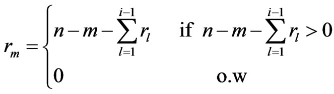
Based on the above data, a progressive first-failure censored data with binomial removals were generated using the algorithm described in Balakrishnan and Sandhu [14] with distribution function  see Wu and Kuş [2].
The generated progressive first-failure censored data with binomial removals are: (0.115, 0.123, 0.1373, 0.1757, 0.2053, 0.2732, 0.2752, 0.2761, 0.2832, 0.4661), and R = (0, 3, 1, 0, 1, 0, 0, 0, 0, 0) Using the results presented in previous sections, the different point estimates of  and
and  are computed. We denote to the MLEs, estimates using the bootstrap, Bayes estimate relative to SE loss, Bayes estimate relative to LINEX loss, and Bayes estimate relative to GE loss, respectively by
  and
and  The results are displayed in Table 1.
Case II: First-failure censoring data with n ( and
and ).
).
The set of the first-failure censored data are: (0.115, 0.123, 0.1373, 0.1757, 0.2053, 0.2136, 0.2732, 0.2752, 0.2761, 0.2814, 0.2832, 0.3165, 0.3194, 0.4661, 0.8348). Different point estimates of  are computed and the results are listed in Table 1.
Case III: Progressive type II censoring data with binomial removals.
A progressive type II censoring data with binomial removals have been generated from complete sample using the algorithm described in Balakrishnan and Sandhu [14], with ( and
and ). i.e. 50 failure times are observed and 25 failure times are censored using censored scheme
 . The generated data are: (0.115, 0.123, 0.1516, 0.1599, 0.2006, 0.2053, 0.2136, 0.2752, 0.2761, 0.2814, 0.2832, 0.3165, 0.3194, 0.3227, 0.3363, 0.4116, 0.4148, 0.5111, 0.5134, 0.5616, 0.5764, 0.6529, 0.679, 0.7273, 0.7353, 0.7441, 0.7602, 0.7871, 0.8052, 0.8312, 0.8461, 0.8632, 0.8695, 0.9049, 0.9088, 0.9328, 0.9407, 0.9698, 0.9732, 0.9787, 0.9939, 0.9956, 1.0344, 1.0935, 1.1291, 1.2067, 1.2178, 1.5136, 1.7956, 1.8144 ). The results of different Bayes estimates of
  and
and  are also, listed in Table 1.
Case IV: The complete sample data with ( and
and )
)
The results of point estimates of the parameter  and
and  are shown in Table 1.
Based on different type of censoring described above, the 95% credible intervals of  and
and  are obtained using approximate confidence interval (ACI), confidence interval based on bootstrap re-sampling method (Boot CI), and the highest posterior density interval (HPDI). All the results are listed in Table 2.
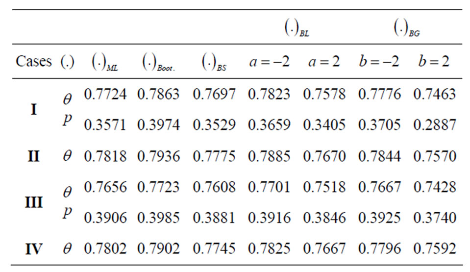
Table 1. Different point estimates of  and
and  for all cases with
 .
.
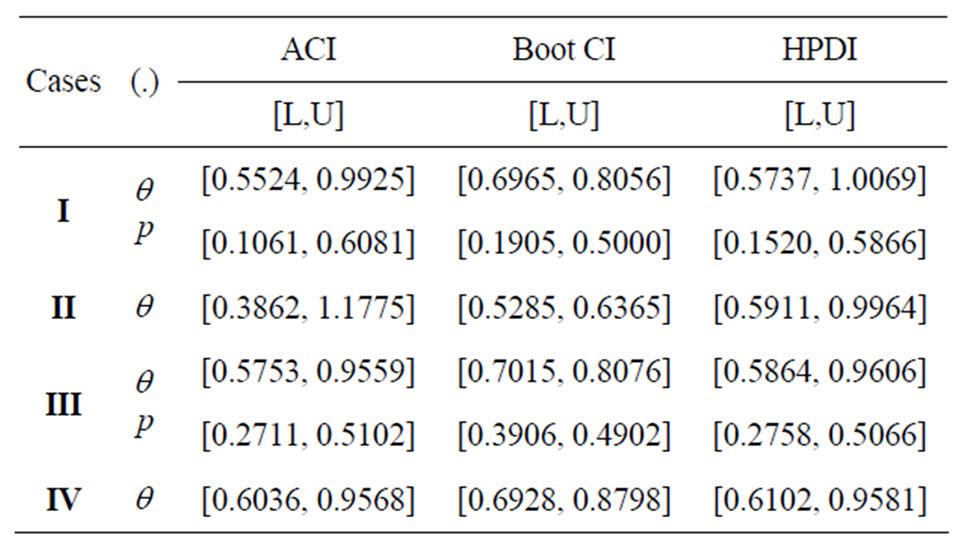
Table 2. 95% confidence intervals for  and
and  under progressive first-failure censored samples when
  .
.
6. Simulation Study
In order to compare the different estimators of the parameters, we simulated  progressively first-failure-censored samples from a Burr type X distribution with the values of parameters
 , and different combinations of
 , and censoring random schemes
  The samples were simulated by using the algorithm described in Balakrishnan and Sandhu [14]. A simulation was conducted in order to study the properties and compare the performance of the Bayes estimator with maximum likelihood estimator.
The mean square error (MSE) of the Bayes estimations and maximum likelihood estimations are computed over different combination of the censored random scheme  as shown in Tables 3 and 4. To asses the effect of the shape parameters a and b from Tables 3 and 4, one can see that the asymmetric Bayes estimates (BL, BG) of the (MSE) of the parameters
  and
and are overestimates for (
 ), and when (
 ) the (MSE) of the parameters are underestimates. Also, the MSE of Bayes estimates are smaller than MSE of the MLE, when
  the MSE of Bayes estimates relative to
  loss are the same as the MSE relative to SE loss Bayes estimates. As anticipated, all MSE of Bayes estimates
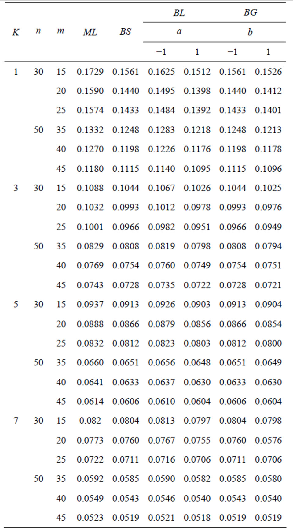
Table 3. Mean square errors of the parameter .
.
relative to both LINEX loss, and GE loss (for  close to 0, and
 ) are the same as the SE loss Bayes estimates. This one of the useful properties of working with the LINEX loss function we found that for different choices of
 ,
,  ,
,  and censoring random scheme
  the MSE of the Bayes estimates based on symmetric and asymmetric loss functions perform better than MSE of the MLEs. when the effective sample proportion
  increases, the MSE of each the Bayes estimation and maximum likelihood estimations reduce. Also the censoring scheme
  is most efficient For all choices, it seems to usually provide the smallest MSE for each estimates of
  and
and .
.
7. Conclusion
The purpose of this paper is to develop a Bayesian analy-

Table 4. Mean square errors of the parameter .
.
sis for Burr-X distribution under the progressively firstfialure censored sampling plan with binomial random removals. We studied point and interval estimations of parameter of the Burr type X distribution. We derived the MLEs, Bayes estimators (BS, BL, BG). A simulation study was conducted to examine the performance of the MLE and the Bayes estimators.
8. Acknowledgements
The authors would like to express their thanks to the editor, assistant editor and referees for their useful comments and suggestions on the original version of this manuscript.
REFERENCES
- L. G. Johnson, “Theory and Technique of Variation Research,” Elsevier, Amsterdam, 1964.
- S.-J. Wu and C. Kus, “On Estimation Based on Progressive First-Failure-Censored Sampling,” Computational Statistics and Data Analysis, Vol. 53, No. 10, 2009, pp. 3659-3670. doi:10.1016/j.csda.2009.03.010
- P. L. Gupta, S. Gupta and Ya. Lvin, “Analysis of Failure Time Data by Burr Distribution,” Communication Statistics Theory & Methods, Vol. 25, No. 9, 1996, pp. 2013- 2024. doi:10.1080/03610929608831817
- A. Childs and N. Balakrishnan, “Conditional Inference Procedures for the Laplace Distribution When the Observed Samples Are Progressively Censored,” Metrika, Vol. 52, No. 3, 2000, pp. 253-265. doi:10.1007/s001840000092
- S. K. Tse, C. Y. Yang and H.-K. Yuen, “Statistical Analysis of Weibull Distribution Lifetime Data under Type II Progressive Censoring with Binomial Removals,” Journal of Applied Statistics, Vol. 27, No. 8, 2000, pp. 1033- 1043. doi:10.1080/02664760050173355
- M. A. M. Ali Mousa and Z. F. Jaheen, “Statistical Inference for the Burr Model Based on Progressively Censored Data,” An International Computers & Mathematics with Applications, Vol. 43, No. 10-11, 2002, pp. 1441-1449. doi:10.1016/S0898-1221(02)00110-4
- K. Ng, P. S. Chan and N. Balakrishnan, “Estimation of Parameters from Progressively Censored Data Using an Algorithm,” Computational Statistics and Data Analysis, Vol. 39, No. 4, 2002, pp. 371-386. doi:10.1016/S0167-9473(01)00091-3
- S.-J. Wu and C.-T. Chang, “Parameter Estimation Based on Exponential Progressive Type II Censored Data with Binomial Removals,” Information and Mangement Statistics, Vol. 13, No. 3, 2002, pp. 37-46.
- N. Balakrishnan, N. Knnan, C. T. Lin and H. Ng, “Point and Interval Estimation for Gaussian Distribution Based on Progressively Type-II Censored Samples,” IEEE Transactions on Reliability, Vol. 52, No. 3, 2003, pp. 90-95. doi:10.1109/TR.2002.805786
- S.-J. Wu, “Estimation for the Two-Parameter Pareto Distribution under Progressive Censoring with Uniform Removals,” Journal of Statistical Computation and Simulation, Vol. 73, No. 2, 2003, pp. 125-134. doi:10.1080/00949650215732
- A. A. Soliman, “Estimation of Parameters of Life from Progressively Censored Data Using Burr-XII Model,” IEEE Transactions on Reliability, Vol. 54, No. 1, 2005, pp. 34-42. doi:10.1109/TR.2004.842528
- A. M. Sarhan and A. Abuammoh, “Statistical Inference Using Progressively Type-II Censored Data with Random Scheme,” International Mathematical Forum, Vol. 35, No. 3, 2008, pp. 1713-1725.
- B. Efron, “The Bootstrap and Other Resampling Plans,” CBMS-NSF Regional Conference Seriesin Applied Mathematics, Vol. 38, SIAM, Philadelphia, 1982.
- N. Balakrishnan and R. Asandhu, “A Simple Simulation Algorithm for Generating Progressively Type-II Censored Samples,” The American Statistican, Vol. 49, No. 2, 1995, pp. 229-230.
- A. P. Basu and N. Ebrahimi, “Bayesian Approach to Life Testing and Reliability Estimation Using Asymmetric Loss Function,” Journal of Statistical Planning and Inference, Vol. 29, No. 1-2, 1991, pp. 21-31. doi:10.1016/0378-3758(92)90118-C
- R. V. Caneld, “A Bayesian Approach to Reliability Estimation Using a Loss Function,” IEEE Transactions on Reliability, Vol. 19, No. 1, 1970, pp. 13-16.
- W. J. Zimmer, J. Bert Keats and F. K. Wang, “The Burr XII Distribution in Reliability Analysis,” Journal of Quality & Technology, Vol. 30, No. 4, 1998, pp. 386-394.
- U. Balasooriya and N. Balakrishnan, “Reliability Sampling Plans for Log-Normal Distribution Based on Progressively Censored Samples,” IEEE Transactions on Reliability, Vol. 49, No. 2, 2000, pp. 199-203. doi:10.1109/24.877338
- A. A. Soliman, “Comparison of LINEX and Quadratic Bayes Estimators for the Rayleigh Distribution,” Communications in Statistics Theory and Methods, Vol. 29, No. 1, 2000, pp. 95-107. doi:10.1080/03610920008832471
- A. A. Soliman, “Estimation of Parameters of Life from Progressively Censored Data Using Burr-XII Model,” IEEE Transactions on Reliability, Vol. 54, No. 1, 2005, pp. 34- 42.
- D. K. Dey, M. Ghosh and C. Srinivasan, “Simultaneous Estimation of Parameters under Entropy Loss,” Journal of Statistical Planning and Inference, Vol. 15, No. 2, 1987, pp. 347-363.
- D. K. Dey and P. L. Liu, “On Comparison of Estimation in Generalized Life Model,” Microelectron & Reliability, Vol. 32, No. 1-2, 1992, pp. 207-221. doi:10.1016/0026-2714(92)90099-7
NOTES
*Mathematics Subject Classification: 62No5; 62F10.