Intelligent Information Management
Vol.3 No.5(2011), Article ID:7187,11 pages DOI:10.4236/iim.2011.35021
Bayesian Inference and Prediction of Burr Type XII Distribution for Progressive First Failure Censored Sampling
Mathematics Department, Sohag University, Sohag, Egypt
E-mail: ahmhamed@hotmail.com
Received April 27, 2011; revised July 16, 2011; accepted July 25, 2011
Keywords: Burr type XII distribution, progressive first-failure censored sample, Bayesian estimations, Gibbs sampling, Markov chain Monte Carlo, Posterior predictive density
Abstract
This paper deals with Bayesian inference and prediction problems of the Burr type XII distribution based on progressive first failure censored data. We consider the Bayesian inference under a squared error loss function. We propose to apply Gibbs sampling procedure to draw Markov Chain Monte Carlo (MCMC) samples, and they have in turn, been used to compute the Bayes estimates with the help of importance sampling technique. We have performed a simulation study in order to compare the proposed Bayes estimators with the maximum likelihood estimators. We further consider two sample Bayes prediction to predicting future order statistics and upper record values from Burr type XII distribution based on progressive first failure censored data. The predictive densities are obtained and used to determine prediction intervals for unobserved order statistics and upper record values. A real life data set is used to illustrate the results derived.
1. Introduction
Censoring is common in life-distribution work because of time limits and other restrictions on data collection. Censoring occurs when exact lifetimes are known only for a portion of the individuals or units under study, while for the remainder of the lifetimes information on them is partial. There are several types of censored tests. One of the most common censored test is type II censoring. It is noted that one can use type II censoring for saving time and money. However, when the lifetimes of products are very high, the experimental time of a type II censoring life test can be still too long. A generalization of Type II censoring is progressive Type II censoring, which is useful when the loss of live test units at points other than the termination point is unavoidable. Recently, the Type-II progressively censoring scheme has received considerable interest among the statisticians. See for example, Kundu [1] and Raqab [2]. For the theory methods and applications of progressive censoring, one can refer to the monograph by Balakrishnan and Aggarwala [3] and the recent survey paper by Balakrishnan [4].
Johnson [5] described a life test in which the experimenter might decide to group the test units into several sets, each as an assembly of test units, and then run all the test units simultaneously until occurrence the first failure in each group. Such a censoring scheme is called a first-failure censoring scheme. Jun et al. [6] discussed a sampling plan for a bearing manufacturer. The bearing test engineer decided to save test time by testing 50 bearings in sets of 10 each. The first-failure times from each group were observed. Wu et al. [7] and Wu and Yu [8] obtained maximum likelihood estimates (MLEs), exact confidence intervals and exact confidence regions for the parameters of the Gompertz and Burr type XII distributions based on first-failure-censored sampling, respectively. If an experimenter desires to remove some sets of test units before observing the first failures in these sets this life test plan is called a progressive first-failure-censoring scheme which recently introduced by Wu and Kuş [9].
In many practical problems of statistics, one wishes to use the results of previous data to predict a future observation from the same population. One way to do this is to construct an interval which will contain the future observation with a specified probability. This interval is called a prediction interval. Prediction has been applied in medicine, engineering, business, and other areas as well. Hahn and Meeker [10] have recently discussed the usefulness of constructing prediction intervals. Bayesian prediction bounds for future observations based on certain distributions have been discussed by several authors. Bayesian prediction bounds for observables having the Burr type XII distribution were obtained by Nigm [11], AL-Hussaini and Jaheen [12,13], and Ali Mousa and Jaheen [14,15]. Burr type X described by Jaheen and AL-Matrafi [16].
Recently, Alamm et al. [17] obtained Bayesian prediction intervals for future order statistics from the generalized exponential distribution. Kundu and Howlader [18] studied Bayesian inference and prediction of inverse Weibull distribution for Type-II censored data. Ahmadi et al. [19] considered the Bayesian prediction of order statistics based on k-record values from exponential distribution. Ahmadi and MirMostafaee [20] obtained prediction intervals for order statistics as well as for the mean life time from a future sample based on observed usual records from an exponential distribution. Ali Mousa and Al-Sagheer [21] discussed the prediction problems for the Rayleigh based on progressively TypeII censored data. The Burr system of distributions includes twelve types of cumulative distribution functions which yield a variety of density shapes and were listed in Burr [22]. Its has applied in business, chemical engineering, quality control, medical and reliability studies.
The probability density function (pdf) and cumulative distribution function (cdf) of the Burr type XII distribution denoted by Burr  are given, respectively, by
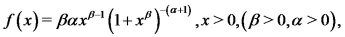 (1)
(1)
and
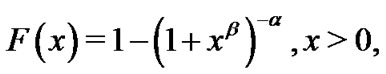 (2)
(2)
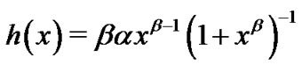
The two-parameter Burr type XII distribution has unimodal or decreasing failure rate function
 . It is clear that the parameter
![]() does not affect the shape of failure rate function
does not affect the shape of failure rate function  and
and  is the shape parameter. Also,
  has a unimodal curve when
  achieving a maximum at
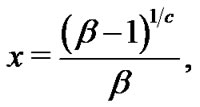 and it has decreasing failure rate function when
 . Thus the shape parameter
  plays an important role for the distribution. Its capacity to assume various shapes often permits a good fit when used to describe biological, clinical or other experimental data. Rodriguez [23] introduced the basic statistical property of Burr type XII model. Lee et al. [24] obtained the Bayes and empirical Bayes estimators of reliability performances of this model under progressively type-II censored samples.
In this paper first we consider the Bayesian inference of the shape parameters for progressive first failure censored data when both parameters are unknown. We assumed that the shape parameters  and
and ![]() have the gamma prior and they are independently distributed. As expected in this case also, the Bayes estimates can not be obtained in closed form. We propose to use the Gibbs sampling procedure to generate MCMC samples, and then using the importance sampling methodology, we obtain the Bayes estimates of the unknown parameters. We perform some simulation experiments to see the behavior of the proposed Bayes estimators and compare their performances with the maximum likelihood estimators (MLEs).
have the gamma prior and they are independently distributed. As expected in this case also, the Bayes estimates can not be obtained in closed form. We propose to use the Gibbs sampling procedure to generate MCMC samples, and then using the importance sampling methodology, we obtain the Bayes estimates of the unknown parameters. We perform some simulation experiments to see the behavior of the proposed Bayes estimators and compare their performances with the maximum likelihood estimators (MLEs).
Another important problem in life-testing experiments namely the prediction of unknown observables belonging to a future sample, based on the current available sample, known in the literature as the informative sample. For different application areas and for references, the readers are referred to AL-Hussaini [25]. In this paper we consider the prediction problem in terms of the estimation of the posterior predictive density of a future observation for two-sample prediction. We also construct predictive interval for a future observation using Gibbs sampling procedure. An illustrative example has been provided.
The rest of this paper is organized as follows: In Section 2, we describe the formulation of a progressive first-failure-censoring scheme. In Section 3, we cover Bayes estimates of parameters using MCMC technique with the help of importance sampling technique. Monte Carlo simulation results are presented in Section 4. Bayes prediction for future order statistic and upper record values are provided in Section 5. and Section 6, respectively. Data analysis is provided in Section 7, and finally we conclude the paper in Section 8.
2. A Progressive First-Failure-Censoring Scheme
In this section, first-failure censoring is combined with progressive censoring as in Wu and Kuş [9]. Suppose that ![]() independent groups with
independent groups with  items within each group are put on a life test,
  groups and the group in which the first failure is observed are randomly removed from the test as soon as the first failure (say
 ) has occurred,
  groups and the group in which the second first failure is observed are randomly removed from the test when the second failure (say
 ) has occurred, and finally
  groups and the group in which the
  first failure is observed are randomly removed from the test as soon as the m-th failure (say
 ) has occurred. The
  are called progressively first-failure-censored order statistics with the progressive censoring scheme
  . It is clear that
 ![]() is number of the first failure observed
is number of the first failure observed  and
and  . If the failure times of the
  items originally in the test are from a continuous population with distribution function
  and probability density function
 , the joint probability density function for
  is given by
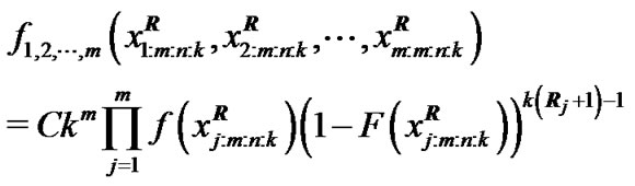 (3)
(3)
 (4)
(4)
where
 (5)
(5)
Special cases
It is clear from (3) that the progressive first-failure censored scheme containing the following censoring schemes as special cases:
1) The first-failure censored scheme when  .
.
2) The progressive type II censored order statistics if .
.
3) Usually type II censored order statistics when  and
and .
.
4) The order statistics case when  and
and  .
.
Also, It should be noted that  can be viewed as a progressive type II censored sample from a population with distribution function
 . For this reason, results for progressive type II censored order statistics can be extend to progressive first-failure censored order statistics easily. Also, the progressive first-failure-censored plan has advantages in terms of reducing the test time, in which more items are used, but only
 ![]() of
of  items are failures.
3. Bayes Estimation
In this section, we present the posterior densities of the parameters  and
and ![]() based on progressively first failure censored data and then obtain the corresponding Bayes estimates of these parameters. To obtain the joint posterior density of
based on progressively first failure censored data and then obtain the corresponding Bayes estimates of these parameters. To obtain the joint posterior density of  and
and![]() , we assume that
, we assume that  and
and ![]() are independently distributed as gamma
are independently distributed as gamma  and gamma
  priors, respectively. Therefore, the prior density functions of
  and
and ![]() becomes
becomes
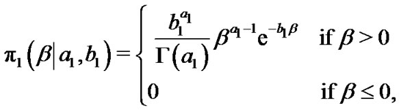 (6)
(6)
 (7)
(7)
The gamma parameters a1, b1, a2 and b2 are all assumed to be positive. When 
 we obtain the non-informative priors of
  and
and![]() .
.
Let ,
,  be the progressively firstfailure-censored order statistics from Burr type XII distribution, with censoring
 . From (3), the likelihood function is given by
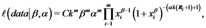 (8)
(8)
where  is defined in (5) and
  is used instead of
 .
.
The joint posterior density function of  and
and ![]() given the data is given by
given the data is given by
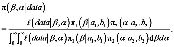 (9)
(9)
Therefore, the posterior density function of  and
and ![]() given the
given the  can be written as
 (10)
(10)
The posterior density (10) can be rewritten as
 (11)
(11)
here, 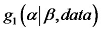 is a gamma density function with the shape and scale parameters as (
 ) and
) and
 , respectively,
  is a proper density function given by
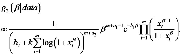 (12)
(12)
Moreover
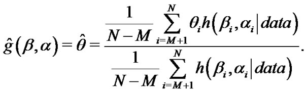
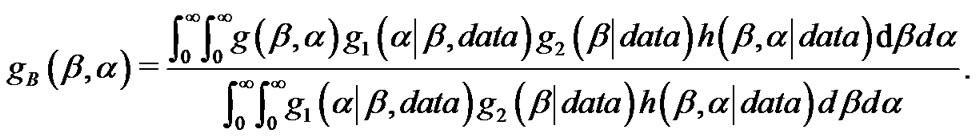
Therefore, the Bayes estimate of any function of  and
and![]() , say
, say  under the squared error loss function is (see Equation (13))
It is not possible to compute (13) analytically. We propose to approximate (13) by using importance sampling technique as suggested by Chen and Shao [26]. The details are explained below.
Importance Sampling
Importance sampling is a useful technique for estimations, now we would like to provide the importance sampling procedure to compute the Bayes estimates for parameters of the Burr type XII distribution, and any function of the parameters say .
.
As mentioned previously that  is a gamma density and, therefore, samples of
 ![]() can be easily generated using any gamma generating routine. However, in our case, the proper density function of
can be easily generated using any gamma generating routine. However, in our case, the proper density function of  Equation (12) cannot be reduced analytically to well known distributions and therefore it is not possible to sample directly by standard methods, but the plot of it (see Figure 1) show that it is similar to normal distribution. So to generate random numbers from this distribution, we use the Metropolis-Hastings method with normal proposal distribution. Using MetropolisHastings method, simulation based consistent estimate of
  can be obtained using Algorithm 1 as given below:
Algorithm 1:
Step 1: Start with an .
.
Step 2: Set .
.
Step 3: Generate  from
from  using the method developed by Metropolis et al. [27] with the N
 proposal distribution.
where  is variances-covariances matrix.
Step 4: Generate  from
from .
.
Step 5: Compute  and
and ![]()
Step 6: Set 
Step 7: Repeat Step 3 - 6 N times and obtain

Figure 1. Posterior density function of β.
 .
.
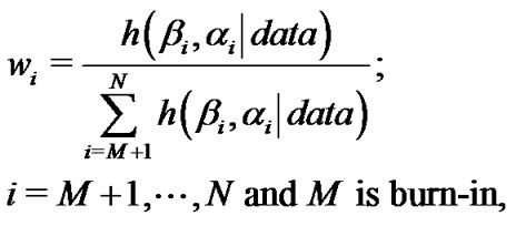
Step 8: An approximate Bayes estimate of  under a squared error loss function can be obtained as
where  is burn-in.
Step 9: Obtain the posterior variance of  as
as

4. Monte Carlo Simulations
In order to compare the proposed Bayes estimators with the MLEs, we perform a Monte Carlo Simulation study using different sample sizes (n), different effective sample sizes (m), different sampling schemes (i.e., different  values) and for different priors (non-informative and informative). We used two sets of parameter values
  and
and  mainly to compare the MLEs and different Bayes estimators and also to explore their effects on different parameter values. For prior information we have used: Non-informative prior, Prior 1 with
 , and informative prior, Prior 2 with
  when
when  and
and  when
when . For Prior 2 we have chosen the hyper-parameters in such a way that the prior mean became the expected value of the corresponding parameter.
It is clear from Tables 1 and 2 that the proposed Bayes
 (13)
(13)
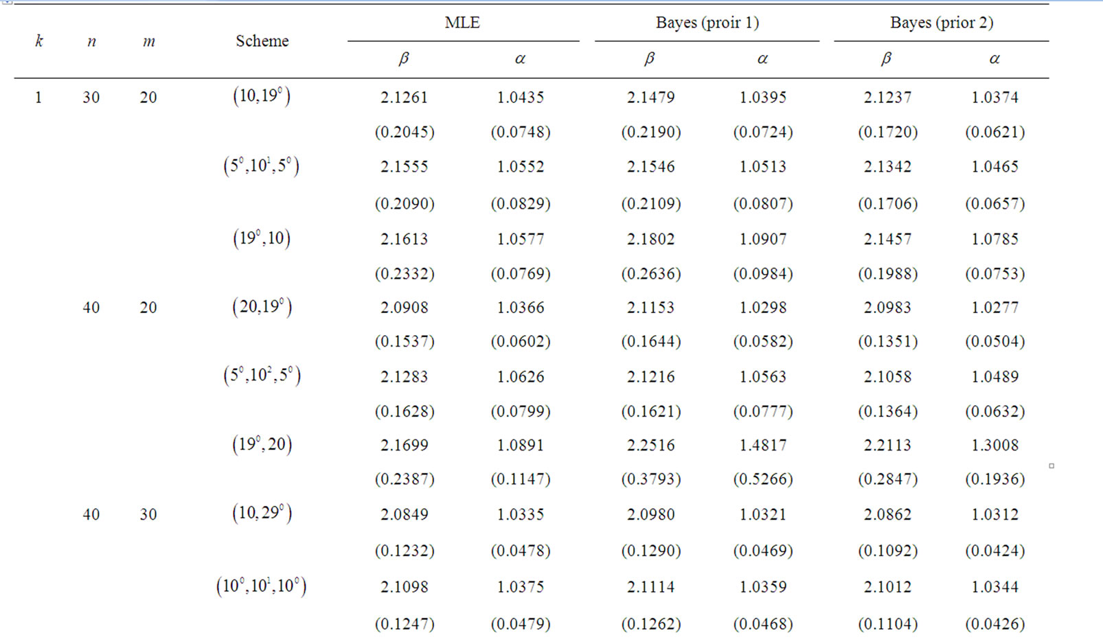
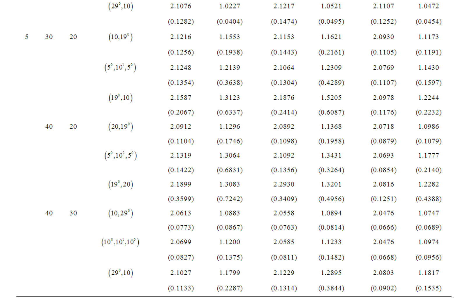
Table 1. Average values of the different estimators and the corresponding MSEs it in parentheses when β = 2 and α = 1.


Table 2. Average values of the different estimators and the corresponding MSEs it in parentheses when β = 1.0 and α = 1.0.
estimators perform very well for different ![]() and
and![]() . As expected, the performance in terms of average and the MSE of the Bayes estimators under Prior 1 and the MLE is very similar. The Bayes estimators under Prior 2 clearly outperform the MLEs in term of average and MSE. Note that prior 2 is more informative than prior 1, because in most cases the MSEs of prior 2 is smaller than that of prior 1.
. As expected, the performance in terms of average and the MSE of the Bayes estimators under Prior 1 and the MLE is very similar. The Bayes estimators under Prior 2 clearly outperform the MLEs in term of average and MSE. Note that prior 2 is more informative than prior 1, because in most cases the MSEs of prior 2 is smaller than that of prior 1.
5. Bayesian Prediction for Future Order Statistics
Suppose that , is a progressive first-failure-censored sample of size
 ![]() drawn from a population whose pdf is Burr
drawn from a population whose pdf is Burr , defined by (1), and that
  is a second independent random sample (of size
![]() ) of future observations from the same distribution. Bayesian prediction bounds are obtained for some order statistics of the future observations
) of future observations from the same distribution. Bayesian prediction bounds are obtained for some order statistics of the future observations . On the other hand, let
  and
and  represent the informative sample from a random sample of size
![]() , and a future ordered sample of size
, and a future ordered sample of size![]() , respectively. It is further assumed that the two samples are independent and each of their corresponding random samples is obtained from the same distribution function. Our aim is to make Bayesian prediction about the
, respectively. It is further assumed that the two samples are independent and each of their corresponding random samples is obtained from the same distribution function. Our aim is to make Bayesian prediction about the ,
,  , ordered lifetime in a future sample of size
![]() .
.
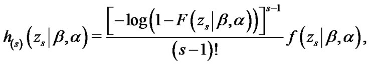
Let  be the
  ordered lifetime in the future sample of size
![]() . The density function of
. The density function of  for given
![]() is of the form
is of the form
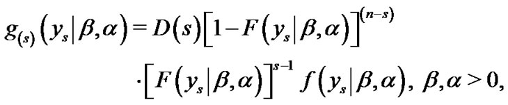 (15)
(15)
where 
here  is given in (1) and
  denotes the corresponding cumulative distribution function of
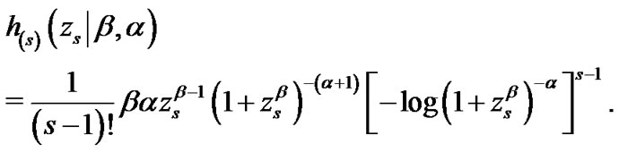
  as given in (2), substituting (1) and (2) in (15), we obtain
 (16)
(16)
where 
By using the binomial expansion, the density (16) takes the form
 (17)
(17)
where
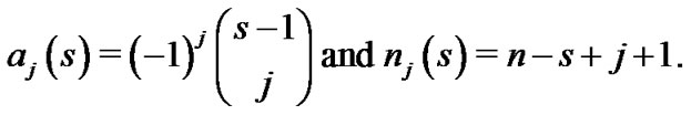 (18)
(18)
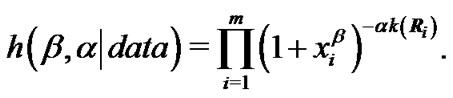
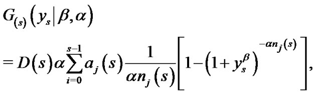
The Bayes predictive density function of  is given by
 (19)
(19)
where  is the joint posterior density of
  and
and ![]() as given in (11). It is immediate that
as given in (11). It is immediate that ![]() can not be expressed in closed form and hence it can not be evaluated analytically.
can not be expressed in closed form and hence it can not be evaluated analytically.
A simulation based consistent estimator of ![]() can be obtained by using the Gibbs sampling procedure as described in Section 3. Suppose
can be obtained by using the Gibbs sampling procedure as described in Section 3. Suppose  are MCMC samples obtained from
  using Gibbs sampling technique, the simulation consistent estimator of
 ![]() can be obtained as
can be obtained as
 (20)
(20)
and a simulation consistent estimator of the predictive distribution of  say
say ![]() can be obtained as
can be obtained as
 (21)
(21)
where
 (22)
(22)
and ![]() denotes the distribution function corresponding to the density function
denotes the distribution function corresponding to the density function ![]() here
here
 (23)
(23)
where  and
and  are defined in (18). It should be noted that the MCMC samples
 can be used to compute
![]() or
or ![]() for all
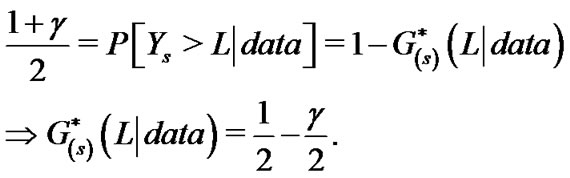
for all . Moreover, a symmetric
  predictive interval for
  can be obtained by solving the non-linear equations (24) and (23), for the lower bound,
 ![]() and upper bound,
and upper bound, 
 (24)
(24)
 (25)
(25)
We need to apply a suitable numerical method as they cannot be solved analytically.
6. Bayesian Prediction for Future Record Value
Let us consider that  is a progressive first failure censored sample of size
 ![]() with progressive censoring scheme
with progressive censoring scheme , drawn from a Burr type XII distribution and let
  is a second independent random sample of size
  of future upper record observations drawn from the same population.
The first sample is referred to as the “informative” (past) sample, while the second one is referred to as the (future) sample. Based on an informative progressively first failure censored sample, our aim is to predict the  upper record values. The conditional pdf of
  for given
  is given see Ahmadi and MirMostafaee [20], by
 (26)
(26)
where  is given in (2) Applying (2) in (26) we obtain
 (27)
(27)
The Bayes predictive density function of  is then
 (28)
(28)
As before, based on MCMC samples  , a simulation consistent estimator of
 ![]() can be obtained as
can be obtained as
 (29)
(29)
and a simulation consistent estimator of the predictive distribution of  say
say ![]() can be obtained as
can be obtained as
 (30)
(30)
 is same as defined in (22) and
 ![]() denotes the distribution function corresponding to the density function
denotes the distribution function corresponding to the density function![]() , we simply obtain
, we simply obtain
 (31)
(31)
It should be noted that the MCMC samples
 can be used to compute
![]() or
or ![]() for all
for all . Moreover, a symmetric
  predictive interval for
  can be obtained by solving the non-linear equations (32) and (33), for the lower bound,
 ![]() and upper bound,
and upper bound, 
 (32)
(32)
 (33)
(33)
In this case also it is not possible to obtain the solutions analytically, and one needs a suitable numerical technique for solving these non-linear equations.
7. Illustrative Example
In this section, we consider a real life data set and illustrate the methods proposed in the previous sections. A complete sample from a clinical trial describe a relief time (in hours) for 50 arthritic patients given by Wingo [28] and used recently by Wu et al. [29] is selected. The data are given in table 3.
Wingo [28] shows that the Burr type XII model is acceptable for these data. To illustrate the use of the estimation methods proposed in this article, we assume that the patients are randomly grouped into 25 groups with  patients within each group. The relief times of the groups are: {0.70, 0.84}, {0.50, 0.58}, {0.55, 0.82}, {0.59, 0.71}, {0.61, 0.72}, {0.49, 0.62}, {0.36, 0.54}, {0.36, 0.71}, {0.35, 0.64}, {0.55, 0.84}, {0.29, 0.59}, {0.46, 0.75}, {0.46, 0.60}, {0.36, 0.60}, {0.52, 0.68}, {0.55, 0.80}, {0.34, 0.84}, {0.34, 0.70}, {0.49, 0.56}, {0.61, 0.71}, {0.57, 0.73}, {0.44, 0.75}, {0.44, 0.81}, {0.8, 0.87}, {0.29, 0.50}. Suppose that the pre-determined progressively first-failure censoring plan is applied using progressive censoring scheme

The following progressively first-failure censored data of size ( ) out of 25 groups of patients were observed: 0.29, 0.29, 0.35, 0.36, 0.36, 0.44, 0.46, 0.46, 0.49, 0.49, 0.5, 0.55, 0.55, 0.55, 0.57, 0.59, 0.61, 0.61, 0.70, 0.80.
For this example, 5 groups of patients are censored, and 20 first failure times are observed. The maximum likelihood estimates (MLE’s) of  and
and  based on complete sample are
  and
and , respectively. Using the progressively first-failure censored sample the MLE's of
  and
and  are 4.5093 and 7.6397, respectively. we apply the Gibbs and Metropolis samplers with the help of importance sampling technique to determine the Bayesian estimation and prediction intervals, we assumed that both the parameters are unknown. Since we do not have any prior information available, we used noninformative priors
  on both
  and
and![]() . The density function of
. The density function of  as given in (12) is plotted Figure 1. It can be approximated by normal distribution function as mentioned in the Subsection 3.1. Now using Algorithm 1, we generate 10,000 MCMC samples and discard the first 1000 values as “burn-in”, based on them we compute the Bayes estimates of
  and
and ![]() as 4.4985 and 7.8716 respectively. As expected the Bayes estimates under the non-informative prior, and the MLE’s are quite close to each other. Moreover, the result of 90% and 95% highest posterior density (HPD) credible intervals of
as 4.4985 and 7.8716 respectively. As expected the Bayes estimates under the non-informative prior, and the MLE’s are quite close to each other. Moreover, the result of 90% and 95% highest posterior density (HPD) credible intervals of  and
and  are given in Tables 4 and 5 for the future order statistics and future upper record values, respectively.
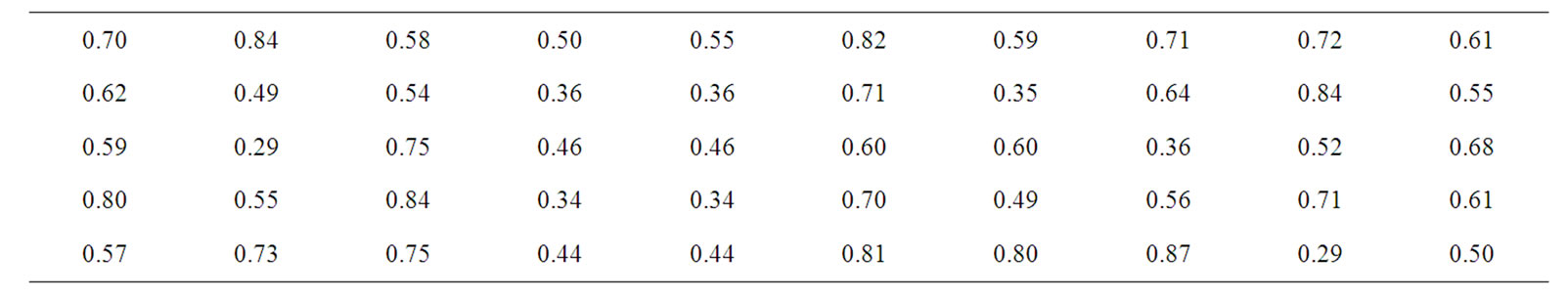
Table 3. Relief time (in hours) for 50 arthritic patients.
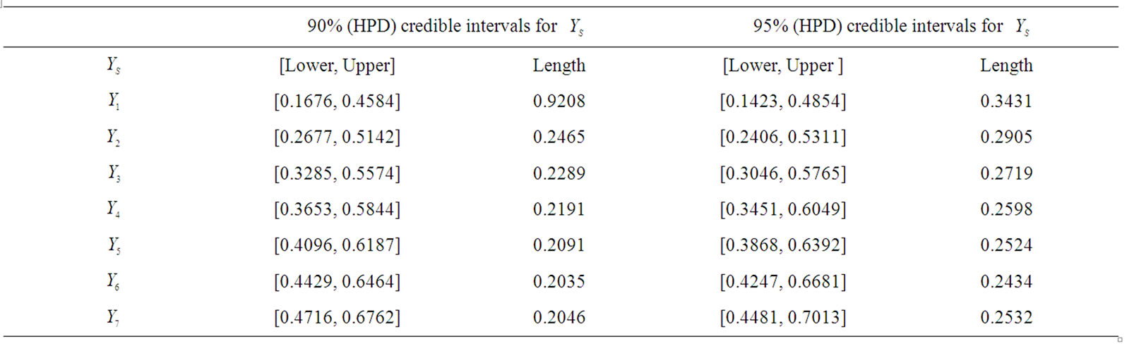
Table 4. Two sample prediction for the future order statistics.
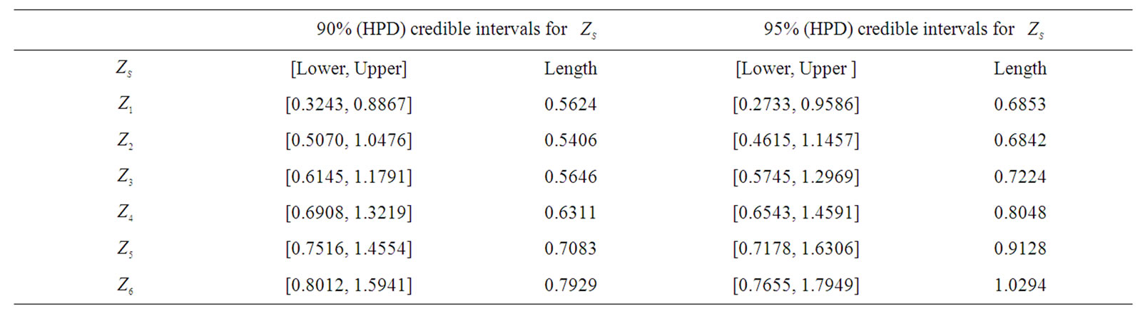
Table 5. Two sample prediction for the future upper record values.
8. Conclusions
In this paper, Bayesian inference and prediction problems of the Burr type XII distribution based on progressive first-failure censored data are obtained for future order statistics and future upper record values. The prior belief of the model is represented by the independent gamma priors on the both shape parameters. The squared error loss function is used. We used Gibbs sampling technique to generate MCMC samples and then using importance sampling methodology we computed the Bayes estimates. The same MCMC samples were used for two sample prediction problems. The details have been explained using a real life example.
9. References
[1] D. Kundu, “Bayesian Inference and Life Testing Plan for the Weibull Distribution in Presence of Progressive Censoring,” Technometrics, Vol. 50, No. 2, 2008, pp. 144- 154. doi:10.1198/004017008000000217
[2] M. Z. Raqab, A. R. Asgharzadeh and R. Valiollahi, “Prediction for Pareto distribution based on progressively Type-II censored samples,” Computational Statistics and Data Analysis,” Vol. 54, No. 7, 2010, pp. 1732-1743. doi:10.1016/j.csda.2010.02.005
[3] N. Balakrishnan and R. Aggarwala, “Progressive Censoring: Theory, Methods, and Applications,” Birkhauser, Boston, 2000.
[4] N. Balakrishnan, “Progressive censoring methodology: An Appraisal,” Test, Vol. 16, No. 2, 2007, pp. 211-296. doi:10.1007/s11749-007-0061-y
[5] L. G. Johnson, “Theory and Technique of Variation Research,” Elsevier, Amsterdam, 1964.
[6] C.-H. Jun, S. Balamurali and S.-H. Lee, “Variables sampling plans for Weibull distributed lifetimes under sudden death testing,” IEEE Transactions on Reliability, Vol. 55, No. 1, 2006, pp. 53-58. doi:10.1109/TR.2005.863802
[7] J.-W. WU, W.-L. Hung and C.-H. Tsai, “Estimation of the parameters of the Gompertz distribution under the first-failure-censored sampling plan,” Statistics, Vol. 37, No. 6, 2003, pp. 517-525. doi:10.1080/02331880310001598864
[8] J.-W. Wu and H.-Y. Yu, “Statistical inference about the shape parameter of the Burr type XII distribution under the failure-censored sampling plan,” Applied Mathematics and Computation, Vol. 163, No. 1, 2005, pp. 443-482. doi:10.1016/j.amc.2004.02.019
[9] S.-J. Wu and C. Kuş, “On Estimation Based on Progressive First-Failure-Censored Sampling,” Computational Statistics and Data Analysis, Vol. 53, No. 10, 2009, pp. 3659-3670. doi:10.1016/j.csda.2009.03.010
[10] G. J. Hahn and W. Q. Meeker, “Statistical Intervals: A Guide for Practitioners,” John Wiley and Sons, Hoboken, 1991.
[11] A. M. Nigm, “Prediction Bounds for the Burr Model,” Communications in Statistics-Theory and Methods, Vol. 17, No. 1, 1988, pp. 287-297. doi:10.1080/03610928808829622
[12] E. K. AL-Huesaini and Z. F. Jaheen, “Bayesian prediction bounds for the Burr type Xll failure model,” Communications in Statistics-Theory and Methods, Vol. 24, No. 7, 1995, pp. 1829-1842. doi:10.1080/03610929508831589
[13] E. K. AL-Huesaini and Z. F. Jaheen, “Bayesian prediction bounds for the Burr type XII distribution in the presence of outliers,” Journal of Statistical Planning and Inference, Vol. 55, 1996, pp. 23-37.
[14] M. A. M. Ali Mousa and Z. F. Jaheen, “Bayesian prediction for the Burr type XII model based on doubly censored data,” Statistics, Vol. 48, 1997, pp. 337-344.
[15] M. A. M. Ali Mousa and Z. F. Jaheen, “ Bayesian prediction for the two-paxameter Burr type XII model based on doubly censored data,” Journal of Applied Statistical Science, Vol. 7, No. 2-3, 1998, pp. 103-111.
[16] Z. F. Jaheen and B. N. AL-Matrafi, “Bayesian prediction bounds from the scaled Burr type X model,” Computers and Mathematics with Applications, Vol. 44, No. 5-6, 2002, pp. 587-594. doi:10.1016/S0898-1221(02)00173-6
[17] A. A. Alamm, M. Z. Raqab and M. T. Madi, “Bayesian prediction intervals for future order statistics from the generalized exponential distribution,” journal of the iranian statistical society, Vol. 6, No. 1, 2007, pp. 17-30.
[18] D. Kundu and H. Howlader, “Bayesian inference and prediction of the inverse Weibull distribution for Type-II censored data,” Computational Statistics and Data Analysis, Vol. 54, No. 6, 2010, pp. 1547-1558. doi:10.1016/j.csda.2010.01.003
[19] J. Ahmadi, S. M. T. K. MirMostafaee and N. Balakrishnanb, “Bayesian prediction of order statistics based on k-record values from exponential distribution,” Statistics, Vol. 44, No. 5, 2010, pp. 1-13.
[20] J. Ahmadi and S. M. T. K. MirMostafaee, “Prediction intervals for future records and order statistics coming from two parameter exponential distribution,” Statistics and Probability Letters, Vol. 79, No. 7, 2009, pp. 977- 983. doi:10.1016/j.spl.2008.12.002
[21] M. A. M. Ali Mousa and S. A. AL-Sagheer, “Bayesian Prediction for Progressively Type-II Censored Data from the Rayleigh Model,” Communications in Statistics-Theory and Methods, Vol. 34, No. 12, 2005, pp. 2353-2361. doi:10.1080/03610920500313767
[22] I. W. Burr, “Cumulative frequency functions,” Annals of Mathematical Statistics, Vol. 13, No. 2, 1942, pp. 215-232. doi:10.1214/aoms/1177731607
[23] R. N. Rodriguez, “A Guide to the Burr type XII distributions,” Biometrika, Vol. 64, No. 1, 1977, pp. 129-134. doi:10.1093/biomet/64.1.129
[24] W. C. Lee, J. W. Wu and C. W. Hong, “Assessing the Lifetime Performance Index of Products from Progressively Type II Right Censored Data Using Burr XII Model,” Mathematics and Computers in Simulation, Vol. 79, No. 7, 2009, pp. 2167-2179. doi:10.1016/j.matcom.2008.12.001
[25] E. K. Al-Hussaini, “Predicting observables from a general class of distributions,” Journal of Statistical Planning and Inference, Vol. 79, No. 1, 1999, pp. 79-91. doi:10.1016/S0378-3758(98)00228-6
[26] M.-H. Chen and Q.-M. Shao, “Monte Carlo estimation of Bayesian Credible and HPD intervals,” Journal of Computational and Graphical Statistics, Vol. 8, no. 1, 1999, pp. 69-92. doi:10.2307/1390921
[27] N. Metropolis, A. W. Rosenbluth, M. N. Rosenbluth, A. H. Teller and E. Teller, “Equations of state calculations by fast computing machines,” Journal Chemical Physics, Vol. 21, No. 6, 1953, pp. 1087-1091. doi:10.1063/1.1699114
[28] D. R. Wingo, “Maximum likelihood methods for fitting the Burr type XII distribution to life test data,” Metrika, Vol. 40, No. 1, 1993, pp. 203-210.
[29] S.-F. Wu, C.-C. Wu, Y.-L. Chen, Y.-R. Yu and Y. P. Lin, “Interval estimation of a two-parameter Burr-XII distribution under progressive censoring,” Statistics, Vol. 44, No. 1, 2010, pp. 77-88. doi:10.1080/02331880902757922