Intelligent Information Management
Vol.2 No.6(2010), Article ID:2017,11 pages DOI:10.4236/iim.2010.26043
Intelligent Optimization Methods for High-Dimensional Data Classification for Support Vector Machines
1College of Computer Science and Technology, Wuhan University of Science and Technology, Wuhan, China
2School of Remote Sensing and Information Engineering, Wuhan University, Wuhan, China
E-mail: dingwhu@gmail.com
Received March 2, 2010; revised April 3, 2010; accepted May 4, 2010
Keywords: support vector machine (SVM), genetic algorithm (GA), particle swarm optimization (PSO), feature selection, optimization
Abstract
Support vector machine (SVM) is a popular pattern classification method with many application areas. SVM shows its outstanding performance in high-dimensional data classification. In the process of classification, SVM kernel parameter setting during the SVM training procedure, along with the feature selection significantly influences the classification accuracy. This paper proposes two novel intelligent optimization methods, which simultaneously determines the parameter values while discovering a subset of features to increase SVM classification accuracy. The study focuses on two evolutionary computing approaches to optimize the parameters of SVM: particle swarm optimization (PSO) and genetic algorithm (GA). And we combine above the two intelligent optimization methods with SVM to choose appropriate subset features and SVM parameters, which are termed GA-FSSVM (Genetic Algorithm-Feature Selection Support Vector Machines) and PSO-FSSVM (Particle Swarm Optimization-Feature Selection Support Vector Machines) models. Experimental results demonstrate that the classification accuracy by our proposed methods outperforms traditional grid search approach and many other approaches. Moreover, the result indicates that PSO-FSSVM can obtain higher classification accuracy than GA-FSSVM classification for hyperspectral data.
1. Introduction
Support vector machine (SVM) was first proposed by Vapnik [1] and has recently been applied in a range of problems including pattern recognition, bioinformatics and text categorization. SVM classifies data with different class labels by determining a set of support vectors that are members of the set of training inputs that outline a hyperplane in the feature space. When using SVM, two issues should be solved: how to choose the optimal input feature subset for SVM, and how to set the best kernel parameters. Traditionally, the two issues are solved separately ignoring their close connections, this always leads low classification accuracy. These two problems are crucial, because the feature subset choice influences the appropriate kernel parameters and vice versa [2]. Therefore, obtaining the optimal feature subset and SVM parameters must occur simultaneously.
Feature selection is used to identify a powerfully predictive subset of fields within a database and reduce the number of fields presented to the mining process. By extracting as much information as possible from a given data set while using the smallest number of features, we can save significant computational time and build models that generalize better for unseen data points. Feature subset selection is an important issue in building an SVM-based classification model.
As well as feature selection, the proper setting of parameters for the SVM classifier can also increase classification accuracy. The parameters that should be optimized include penalty parameter C and the kernel function parameters such as the gamma (γ) for the radial basis function (RBF) kernel. To design a SVM classifier, one must choose a kernel function, set the kernel parameters and determine a soft margin constant C (penalty parameter). As a rule, the Grid algorithm is an alternative to finding the best C and gamma (γ) when using the RBF kernel function. However, this method is time consuming and does not perform well [3]. Moreover, the Grid algorithm can not perform the feature selection task.
Both feature subset selection and model parameter setting substantially influence classification accuracy. The optimal feature subset and model parameters must be determined simultaneously. Since feature subset and model parameters greatly affects the classification accuracy.
To simultaneously optimize the feature subset and the SVM kernel parameters, this study attempts to increase the classification accuracy rate by employing two evolutionary computing optimization-based approaches: genetic algorithm (GA) and particle swarm optimization (PSO) in SVM. These novel approaches are termed PSO-FSSVM (Particle Swarm Optimization-Feature Selection Support Vector Machines) and GA-FSSVM (Genetic Algorithm-Feature Selection Support Vector Machines). The developed approaches not only tune the parameter values of SVM, but also identify a subset of features for specific problems, maximizing the classification accuracy rate of SVM. This makes the optimal separating hyperplane obtainable in both linear and non-linear classification problems.
The remainder of this paper is organized as follows. Section 2 reviews pertinent literature on SVM and the feature selection. Section 3 then describes basic GA concept and GA-FSSVM model of feature selection and parameter optimization. Also, Section 3 then describes in detail the developed PSO-FSSVM approach for determining the parameter values for SVM with feature selection. Section 4 compares the experimental results with those of existing traditional approaches. Conclusions are finally drawn in Section 5, along with recommendations for future research.
2. Literature Review
Approaches for feature selection can be categorized into two models, namely a filter model and a wrapper model [4]. Statistical techniques, such as principal component analysis, factor analysis, independent component analysis and discriminate analysis can be adopted in filterbased feature selection approaches to investigate other indirect performance measures, most of which are based on distance and information. Chen and Hsieh [5] presented latent semantic analysis and web page feature selection, which are combined with the SVM technique to extract features. Gold [6] presented a Bayesian viewpoint of SVM classifiers to tune hyper-parameter values in order to determine useful criteria for pruning irrelevant features.
The wrapper model [7] applies the classifier accuracy rate as the performance measure. Some researchers have concluded that if the purpose of the model is to minimize the classifier error rate, and the measurement cost for all the features is equal, then the classifier’s predictive accuracy is the most important factor. Restated, the classifier should be constructed to achieve the highest classification accuracy. The features adopted by the classifier are then chosen as the optimal features. In the wrapper model, meta-heuristic approaches are commonly employed to help in looking for the best feature subset. Although meta-heuristic approaches are slow, they obtain the (near) best feature subset. Shon [8] employed GA to screen the features of a dataset. The selected subset of features is then fed into the SVM for classification testing. Zhang [9] developed a GA-based approach to discover a beneficial subset of features for SVM in machine condition monitoring. Samanta [10] proposed a GA approach to modify the RBF width parameter of SVM with feature selection. Nevertheless, since these approaches only consider the RBF width parameter for the SVM, they may miss the optimal parameter setting. Huang and Wang [11] presented a GA-based feature selection and parameters optimization for SVM. Moreover, Huang et al. [12] utilized the GA-based feature selection and parameter optimization for credit scoring.
Several kernel functions help the SVM obtain the optimal solution. The most frequently used such kernel functions are the polynomial, sigmoid and radial basis kernel function (RBF). The RBF is generally applied most frequently, because it can classify high-dimensional data, unlike a linear kernel function. Additionally, the RBF has fewer parameters to set than a polynomial kernel. RBF and other kernel functions have similar overall performance. Consequently, RBF is an effective option for kernel function. Therefore, this study applies an RBF kernel function in the SVM to obtain optimal solution. Two major RBF parameters applied in SVM, C and γ, must be set appropriately. Parameter C represents the cost of the penalty. The choice of value for C influences on the classification outcome. If C is too large, then the classification accuracy rate is very high in the training phase, but very low in the testing phase. If C is too small, then the classification accuracy rate is unsatisfactory, making the model useless. Parameter γ has a much greater influence on classification outcomes than C, because its value affects the partitioning outcome in the feature space. An excessively large value for parameter γ results in over-fitting, while a disproportionately small value leads to under-fitting. Grid search [13] is the most common method to determine appropriate values for C and γ. Values for parameters C and γ that lead to the highest classification accuracy rate in this interval can be found by setting appropriate values for the upper and lower bounds (the search interval) and the jumping interval in the search. Nevertheless, this approach is a local search method, and vulnerable to local optima. Additionally, setting the search interval is a problem. Too large a search interval wastes computational resource, while too small a search interval might render a satisfactory outcome impossible.
In addition to the commonly used grid search approach, other techniques are employed in SVM to improve the possibility of a correct choice of parameter values. Pai and Hong [14] proposed an SA-based approach to obtain parameter values for SVM, and applied it in real data; however, this approach does not address feature selection, and therefore may exclude the optimal result. As well as the two parameters C and γ, other factors, such as the quality of the feature’s dataset, may influence the classification accuracy rate. For instance, the correlations between features influence the classification result. Accidental removal of important features might lower the classification accuracy rate. Additionally, some dataset features may have no influence at all, or may contain a high level of noise. Removing such features can improve the searching speed and accuracy rate.
It is worth underlining that the kernel-based implementation of SVM involves the problem of the selection of multiple parameters, including the kernel parameters (e.g., the γ and p parameters for the Gaussian and polynomial kernels, respectively) and the regularization parameters C.
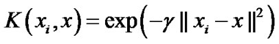
Studies have also illustrated that a radial basis kernel yields the best results in remote sensing applications [15, 16]. We chose to use the radial basis kernel for SVM in this study. The verification of the applicability of other specialized kernel functions for the classification of remote sensing data may be used in future studies. The equation for the radial basis kernel is
 (1)
(1)
where γ represents a parameter inversely proportional to the width of the Gaussian kernel.
3. The Proposed GA-FSSVM and PSO-FSSVM Models
3.1. Genetic Algorithm
The genetic algorithms are inspired by theory of evolution; it is type of an evolutionary computing. The problems are solved by an evolutionary process resulting in a fittest solution in genetic algorithm. A genetic algorithm (GA) is used to solve global optimization problems. The procedure starts from a set of randomly created or selected possible solutions, referred to as the population. Every individual in the population means a possible solution, referred to as a chromosome. Within every generation, a fitness function should be used to evaluate the quality of every chromosome to determine the probability of it surviving to the next generation; usually, the chromosomes with larger fitness have a higher survival probability. Thus, GA should select the chromosomes with larger fitness for reproduction by using operations like selection, crossover and mutation in order to form a new group of chromosomes which are more likely to reach the goal. This reproduction goes through one generation to another, until it converges on the individual generation with the most fitness for goal functions or the required number of generations was reached. The optimal solution is then determined.
GA coding strategies mainly include two sectors: one sector recommends the least digits for coding usage, such as binary codes, another one recommends using the real-valued coding based on calculation convenience and accuracy. Binary codes are adopted for the decision variables in solving the discrete problems, a suitable encoding scheme is needed to encode the chromosome of each individual, in our study, an encoding scheme is usually a binary string. We may define the length of bit string according the precision.
3.2. GA-FSSVM Model
As mentioned before, a kernel function is required in SVM for transforming the training data. This study adopts RBF as the kernel function to establish support vector classifiers, since the classification performance is significant when the knowledge concerning the data set is lacking. Therefore, there are two parameters, C and γ, required within the SVM algorithm for accurate settings, since they are closely related to the learning and predicting performance. However, determining the values exactly is difficult for SVM. Generally, to find the best C and γ, a given parameter is first fixed, and then within the value ranges another parameter is changed and cross comparison is made using the grid search algorithm. This method is conducted with a series of selections and comparisons, and it will face the problems of lower efficiency and inferior accuracy when conducting a wider search. However, GA for reproduction could provide the solution for this study. The scheme of an integration of GA and SVM is shown in Figure 1, to establish a training and SVM classification model that can be used to determine optimized SVM parameters and subset features mask. Following the above scheme of the proposed GA-FSSVM model, Figure 1 describes the operating procedure in this study.
A fitness function assesses the quality of a solution in the evaluation step. The crossover and mutation functions are the main operators that randomly impact the fitness value. Chromosomes are selected for reproduction by evaluating the fitness value. The fitter chromosomes have higher probability to be selected into the recombination pool using the roulette wheel or the tournament selection methods. New population replaces the old population using the elitism or diversity replacement strategy and forms a new population in the next generation. The evolutionary process operates many generations until termination condition is satisfied.

Figure 1. system architecture of the integrated GA-FSSVM scheme.
To implement our proposed approach, this research uses the RBF kernel function for the SVM classifier because the RBF kernel function can analysis higher-dimensional data and requires that only two parameters, C and γ be defined When the RBF kernel is selected, the parameters (C and γ) and features used as input attributes must be optimized using our proposed GA-based system. Therefore, the chromosome comprises three parts: C, γ and the features mask. However, these chromosomes have different parameters when other types of kernel functions are selected. The binary coding system is used to represent the chromosome.
Figure 2 shows the binary chromosome representation of our design. In Figure 2,  ~
~ represents the value of parameter C,
  ~
~ represents the parameter value γ, and
  ~
~ represents the feature mask.
  is the number of bits representing parameter C,
  is the number of bits representing parameter g, and
  is the number of bits representing the features. Note that we can choose
  and
and  according to the calculation precision required, and that
  equals the number of features varying from the different datasets. In Figure 2, the bit strings representing the genotype of parameter C and γ should be transformed into phenotype. Note that the precision of representing parameter depends on the
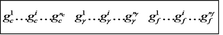
Figure 2. the chromosome comprise three parts: C, γ and the features mask.
length of the bit string, and the minimum and maximum value of the parameter is determined by the user. For chromosome representing the feature mask, the bit with value ‘1’ represents the feature is selected, and ‘0’ indicates feature is not selected. In our study, classification accuracy, the numbers of selected features are the criteria used to design a fitness function. Thus, for the individual with high classification, a small number of features produce a high fitness value.
3.3. Particle Swarm Optimization
Particle swarm optimization (PSO) [17] is an emerging population-based meta-heuristic that simulates social behavior such as birds flocking to a promising position to achieve precise objectives in a multi-dimensional space. Like evolutionary algorithms, PSO performs searches using a population (called swarm) of individuals (called particles) that are updated from iteration to iteration. To discover the optimal solution, each particle changes its searching direction according to two factors, its own best previous experience (pbest) and the best experience of all other members (gbest). They are called pbest the cognition part, and gbest the social part. Each particle represents a candidate position (i.e., solution). A particle is considered as a point in a D-dimension space, and its status is characterized according to its position and velocity. The D-dimensional position for the particle i at iteration t can be represented as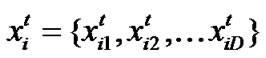 . Likewise, the velocity (i.e., distance change), which is also an D-dimension vector, for particle i at iteration t can be described as
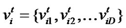 .
.
Let 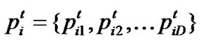 represent the best solution that particle i has obtained until iteration t, and
 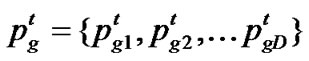 denote the best solution obtained from
 in the population at iteration t. To search for the optimal solution, each particle changes its velocity according to the cognition and social parts as follows:
 (2)
(2)
 (3)
(3)
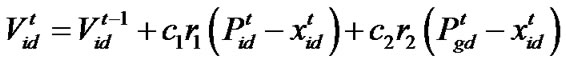
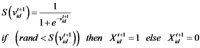
d=1, 2,…, D where c1 indicates the cognition learning factor; c2 indicates the social learning factor, and r1 and r2 are random numbers uniformly distributed in U(0,1). Each particle then moves to a new potential solution based on the following equation: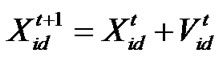 , d = 1, 2,…, D. The basic process of the PSO algorithm is given as follows.
Step 1: (Initialization) Randomly generate initial particles.
Step 2: (Fitness) Measure the fitness of each particle in the population.
Step 3: (Update) Compute the velocity of each particle with Equation (2).
Step 4: (Construction) For each particle, move to the next position according to Equation (3).
Step 5: (Termination) Stop the algorithm if termination criterion is satisfied; return to Step 2 otherwise the iteration is terminated if the number of iteration reaches the pre-determined maximum number of iteration.
Figure 3 shows the flowchart for PSO-SVM classifier.
Based on the rules of particle swarm optimization, we set the required particle number first, and then the initial coding alphabetic string for each particle is randomly produced. In our study, we coded each particle to imitate a chromosome in a genetic algorithm.
3.4. PSO-FSSVM Model
In this following of the section, we describe the proposed SVM-PSO classification system for the classification of high-dimensional data. As mentioned in the Introduction, the aim of this system is to optimize the SVM classifier accuracy by automatically: 1) detecting the subset of the best discriminative features (without requiring a userdefined number of desired features) and 2) solving the SVM-RBF model selection issue (i.e., estimating the best values of the regularization and kernel parameters). In order to attain this, the system is derived from an optimization framework based on PSO.
This study developed a PSO approach, termed PSOFSSVM, for parameter determination and feature selection in the SVM. Without feature selection, two decision variables, designated C and γ are required. For the feature selection, if n features are required to decide which features are chosen, then 2 + n decision variables must be adopted. The value of n variables ranges between 0 and 1. If the value of a variable is less than or equal to 0.5, then its corresponding feature is not chosen. Conversely, if the value of a variable is greater than 0.5, then its corresponding feature is chosen. Figure 4 illustrates the solution representation. Pc = C, Pγ = γ, an = Feature n is selected or not.
The following shows the while process for PSOFSSVM. First, the population of particles is initialized, each particle having a random position within the D-dimensional space and a random velocity for each dimension. Second, each particle’s fitness for the SVM is
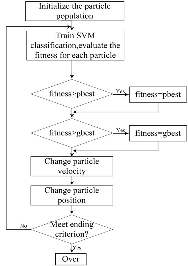
Figure 3. the process of PSO algorithm for solving optimization problems.
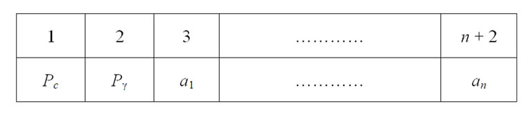
Figure 4. Solution representation.
evaluated. The each particle’s fitness in this study is the classification accuracy. If the fitness is better than the particle’s best fitness, then the position vector is saved for the particle. If the particle’s fitness is better than the global best fitness, then the position vector is saved for the global best. Finally the particle’s velocity and position are updated until the termination condition is satisfied. Figure 5 shows the architecture of the developed PSO-based parameter determination and feature selection approach for SVM.
4. Experimental Results
To evaluate the classification accuracy of the proposed system in different classification tasks, we tried two real-world datasets: the UCI database [18] and hyperspectral benchmark data set [19]. These two data sets have been frequently used as benchmarks to compare the performance of different classification methods in the literature.
Our implementation was carried out on the Matlab 7.0 development environment by extending the LIBSVM
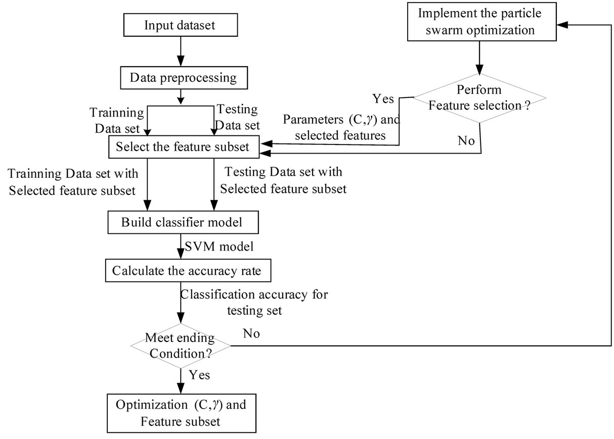
Figure 5. the architecture of the proposed PSD-SVM based parameters determination and feature selection approach for SVM.
which is originally designed by Chang and Lin [20]. The empirical evaluation was performed on Intel Pentium Dual-Core CPU running at 1.6 GHz and 2G RAM.
4.1. UCI Dataset
These UCI datasets consist of numeric and nominal attributes. To guarantee valid results for making predictions regarding new data, the dataset is further randomly partitioned into training sets and independent test sets via a k-fold cross validation. Each of the k subsets acted as an independent holdout test set for the model trained with the remaining k – 1 subsets. The advantages of cross validation are that all of the test sets were independent and the reliability of the results could be improved. The data set is divided into k subsets for cross validation. A typical experiment uses k = 10. Other values may be used according to the data set size. For a small data set, it may be better to set larger k, because this leaves more examples in the training set. This study used k = 10, meaning that all of the data will be divided into 10 parts, each of which will take turns at being the testing data set. The other nine data parts serve as the training data set for adjusting the model prediction parameters.
The Grid search algorithm is a common method for searching for the best C and . Figure 6 shows the process of Grid algorithm combined with SVM classifier. In the Grid algorithm, pairs of (C,
 ) are tried and the one with the best cross-validation accuracy is chosen.
After identifying a ‘better’ region on the grid, a finer grid search on that region can be conducted. This research conducted the experiments using the proposed GA-SVM and PSO-SVM approaches and the Grid algorithm. The results from the proposed method were compared with that from the Grid algorithm. In all of the experiments 10-fold cross validation is used to estimate the accuracy of each learned classifier.
The detail parameter setting for genetic algorithm is as the following: population size 20, crossover rate 0.6, mutation rate 0.05, single-point crossover, roulette wheel selection, and elitism replacement, we set nc = 12, nγ = 15, the value of nf depends on the experimental datasets stated in Table 2. According to the fitness function and the number of selected features, we can compare different methods. The GA-FSSVM and PSO-FSSVM related parameters is described in Table 3.
The termination criterion is that the generation number reaches generation 100. The best chromosome is obtained when the termination criteria satisfy. Taking the German dataset, for example, over accuracy, number of selected features for each fold using GA-FSSVM approach, PSO-FSSVM approach and Grid algorithm are shown in Table 1. For GA-SVM approach, its average accuracy is 87.08%, and average number of features is 11.46, and for PSO-SVM approach, the average accuracy is 85.47% and average number of features is 10.92, but for Grid algorithm, its average accuracy is 81.46%, and all 24 features are used.
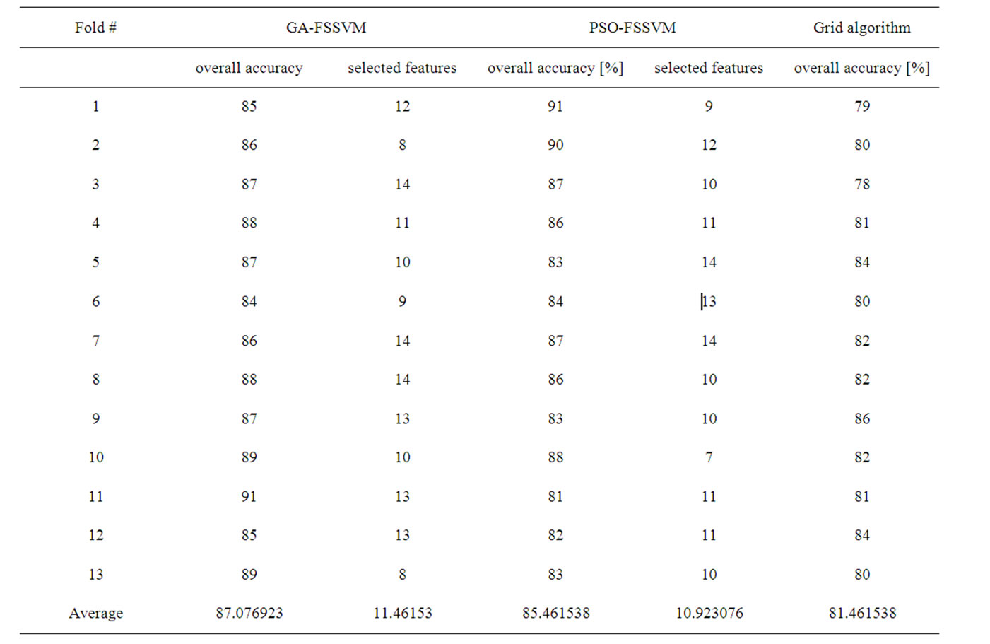
Table 1. Experimental result for German dataset using GA-based, PSO-based and grid algorithm approach.
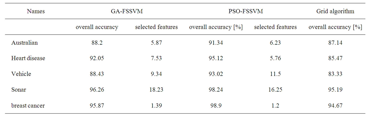
Table 2. Experimental results for test dataset.
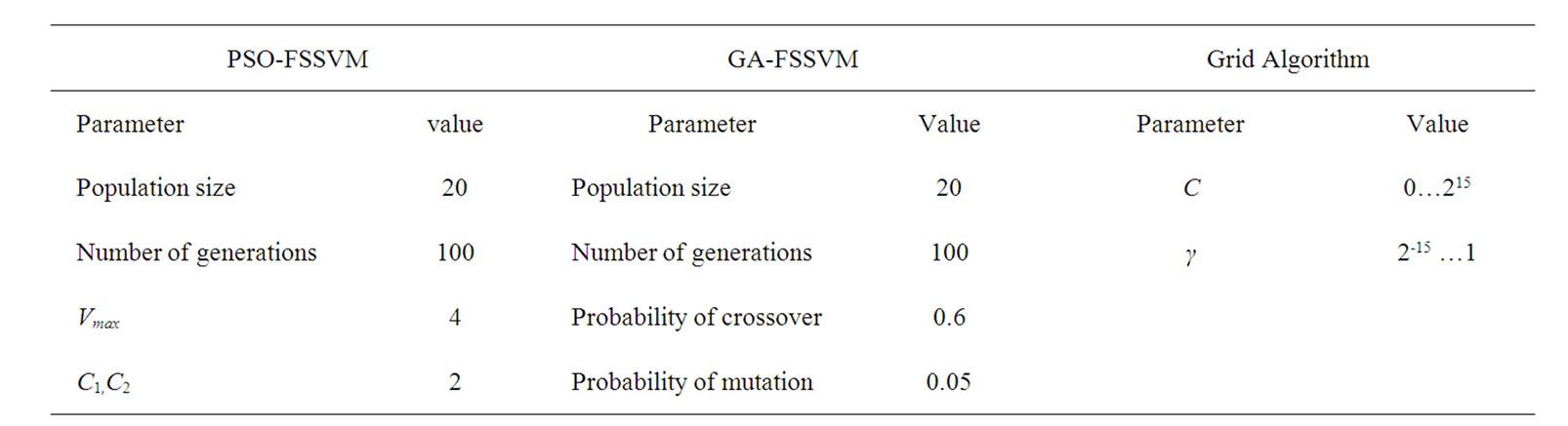
Table 3. Parameters setting.
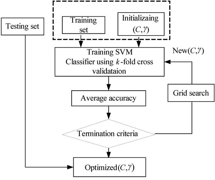
Figure 6. parameters setting using grid algorithm.
To compare the two proposed evolutionary computing approaches with the Grid algorithm, as shown in Table 1. Generally, compared with the Grid algorithm, the two proposed approaches have good accuracy performance with fewer features.
4.2. Hyperspectral Dataset
4.2.1. Dataset Description
To validate the proposed intelligent optimization methods, we also compare the two evolutionary computing methods with traditional classification method for hyperspectral data classification. The classifier is used by SVM.
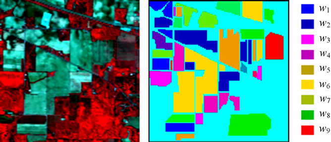
The hyperspectral remote sensing image used in our experiments is a section of a scene taken over northwest Indiana’s Indian Pines by the AVIRIS sensor in 1992 [19]. From the 220 spectral channels acquired by the AVIRIS sensor, 20 channels are discarded because affected by atmospheric problems. From the 16 different land-cover classes available in the original ground truth, seven classes are removed, since only few training samples were available for them (this makes the experimental analysis more significant from the statistical viewpoint). The remaining nine land-cover classes were used to generate a set of 4757 training samples (used for learning the classifiers) and a set of 4588 test samples (exploited for assessing their accuracies) (see Table 4). The origin image and reference image are shown in Figure 7.
4.2.2. Experiment Settings
In the experiments, when using the proposed intelligent optimization methods, we considered the nonlinear SVM based on the popular Gaussian kernel (referred to as SVM-RBF). The related parameters C and γ for this kernel were varied in the arbitrarily fixed ranges [10−3, 300]
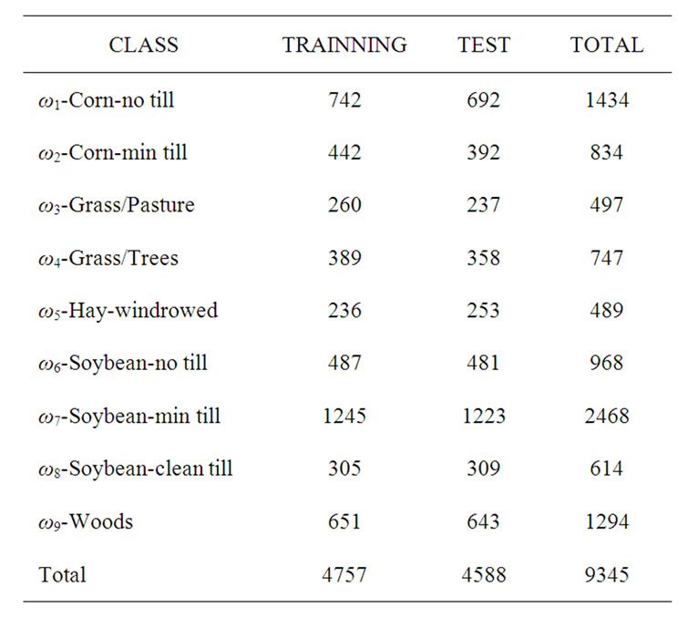
Table 4. Number of training and test samples.
 (a) (b)
Figure 7. hyperspectral image data. (a) Origin image; (b) Ground truth image.
and [10−3, 3], so as to cover high and small regularization of the classification model, and fat as well as thin kernels, respectively. The experiments are implemented by LIBSVM [20].
LIBSVM is widely used in SVM classifier, but the value of RBF kernel parameters is always difficult to define. The default values are as follows: C is 1, and γ is the reciprocal of the dimension. In our experiment, the dimension is the band number, so the parameter value of γ is 0.005.In the same way, the default value of C of SVM parameter in ENVI is 100, and γ is the reciprocal of the dimension. In our experiment, the dimension is the band number, so the parameter value of γ is 0.005. In addition, we also select SVM parameters by grid algorithm. In grid algorithm, according to reference [4], the range of C and γ is [2-5, 215] and [2-15, 23], the step length is 22.
Concerning the PSO algorithm, we considered the following standard parameters: swarm size S = 20, inertia weight w = 1, acceleration constants c1 and c2 equal to 2, and maximum number of iterations fixed at 300. The parameters setting is summarized in Table 5.
In addition, for comparison purpose, we implemented the three traditional methods and our two intelligent optimization methods for classification. The experimental comparison results are shown in Figure 8 and Table 6.
We apply the PSO-FSSVM classifier to the available training data. Note that each particle of the swarm was defined by position and velocity vectors of a dimension of 202. At convergence of the optimization process, we assessed the PSO-FSSVM-RBF classifier accuracy on the test samples. The achieved overall accuracy is 95.25% corresponding to substantial accuracy gains as compared to what is yielded either by the SVM classifier (with the Gaussian kernel) based grid algorithm applied to all available features (+4.27%) or by the GA-FSSVM classifier (+2.36) with 101 features. Moreover, by means of this approach, the average subset feature number is 120, which is fewer than original feature number 220. The whole process is implemented automatically and without user’s interface.
Table 6 illustrates the classification of different classifiers. As can be seen our proposed classifier have better accuracy than traditional classifiers. The LIBSVM default setting lead to the lowest accuracy, which is 52.79%.The best percentage of classification, is 95.25% by PSO-FSSVM method. The results still confirm the strong superiority of our proposed PSO-FSSVM over the other classifiers, with a gain in overall accuracy +12.80%, +4.27% and +2.36% with respect to the default SVM classifier in ENVI, the grid algorithm, and the GA-SVM classifiers (see Table 6).
From the obtained experimental results, we conclude the proposed PSO-FSSVM classifier has the best classification accuracy account of its superior generalization capability as compared to traditional classification techniques.
5. Discussion and Conclusion
Feature selection is an important issue in the construction of classification system. The number of input features in a classifier should be limited to ensure good predictive power without an excessively computationally intensive model. This work investigated two novel intelligent optimization models that hybridized the two evolutionary computing optimizations and support vector machines to maintain the classification accuracy with small and suitable feature subsets. The work is novel, since few researches have conducted on the GA-FSSVM and PSOFSSVM classification system to find simultaneously an optimal feature subset and SVM model parameters in high-dimensional data classification.
In this paper, we addressed the problem of the classification of high dimensional data using intelligent optimization methods. This study presents two evolutionary computing optimization approaches: GA-FSSVM and PSO-FSSVM, capable of searching for the optimal parameter values for SVM and a subset of beneficial features. This optimal subset of features and SVM parameters are then adopted in both training and testing to obtain

Table 5. Parameters setting of different methods.
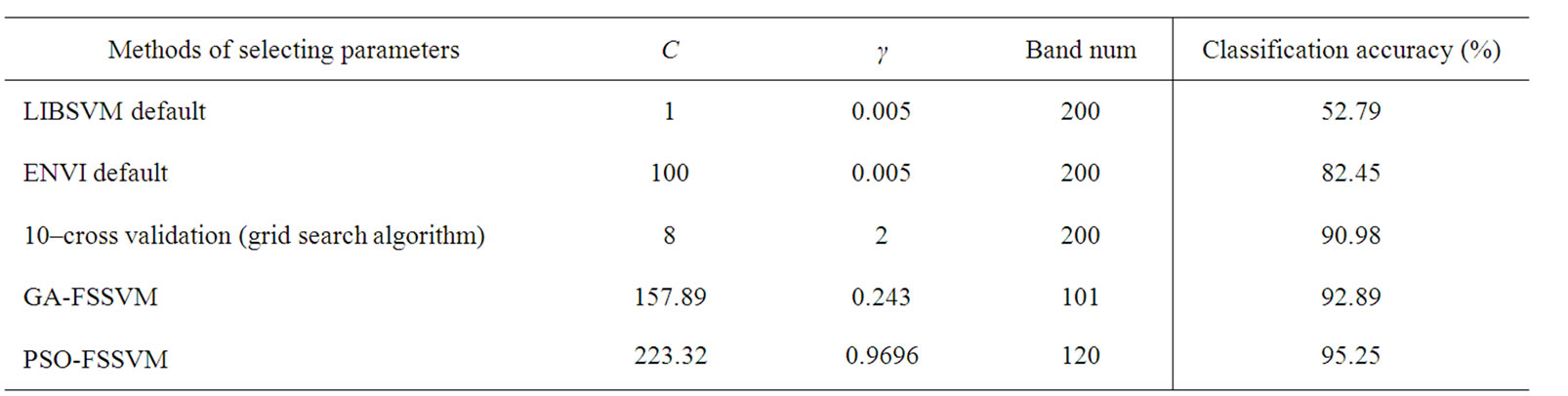
Table 6. Classification result by different parameter selec tion methods.
 (a)
(a)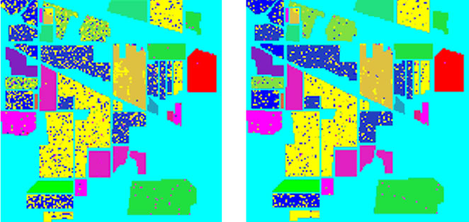 (b)
(b)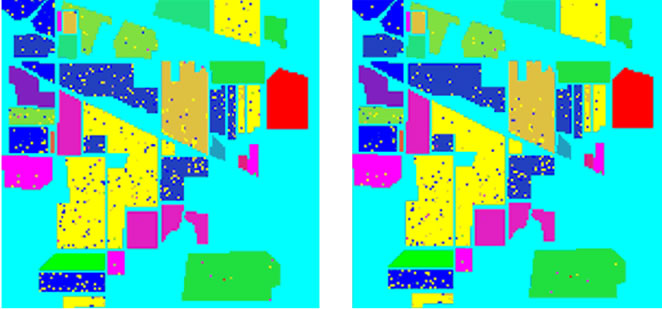 (c)
(c)
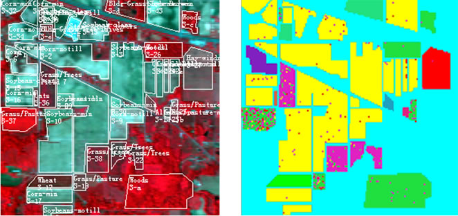
Figure 8. Classification accuracy of different classifiers. (a) Train data and test data; (b) LIBSVM 52.79%; (c) ENVI 82.45%; (d) Grid algorithm 90.98%; (e) GA-FSSVM 92.89%; (f) PSO-FSSVM 95.25%.
the optimal outcomes in classification. Comparison of the obtained results with traditional Grid-based approach demonstrates that the developed PSO-FSSVM and GA-FSSVM approach have better classification accuracy with fewer features. After using feature selection in the experiment, the proposed approaches are applied to eliminate unnecessary or insignificant features, and effectively determine the parameter values, in turn improving the overall classification results, and the PSOFSSVM approach is better than GA-FSSVM in most datasets in our experiments.
Experimental results concerning a simulated dataset revealed that the proposed approach not only optimized the classifier’s model parameters and correctly obtained the discriminating feature subset, but also achieved accurate classification accuracy.
Results of this study are obtained with an RBF kernel function. However, other kernel parameters can also be optimized using the same approach. Experimental results obtained from UCI datasets, other public datasets and real-world problems can be tested in the future to verify and extend this approach.
In the future, we need to further improve the classification accuracy by using other evolutionary optimization algorithm, such as Simulated Annealing Algorithm (SAA), Artificial Immune Algorithm (AIA). In addition, we are to optimize the SVM classifiers by several combinative evolutionary optimization methods in the future.
6. Acknowledgements
The authors would like to thank the anonymous referees for their valuable comments, which helped in improving the quality of the paper. This research was supported by National Natural Science Foundation of China under Grant NO. 60705012.
7. References
[1] V. N. Vapnik, “The Nature of Statistical Learning Theory,” Springer Verlag, New York, 2000.
[2] H. Fröhlich and O. Chapelle, “Feature Selection for Support Vector Machines by Means of Genetic Algorithms,” Proceedings of the 15th IEEE International Conference on Tools with Artificial Intelligence, Sacramento, 3-5 November 2003, pp. 142-148.
[3] C. W. Hsu and C. J. Lin, “A Simple Decomposition Method for Support Vector Machine,” Machine Learning, Vol. 46, No. 3, 2002, pp. 219-314.
[4] H. Liu and H. Motoda, “Feature Selection for Knowledge Discovery and Data Mining,” Kluwer Academic, Boston, 1998.
[5] R. C. Chen and C. H. Hsieh, “Web Page Classification Based on a Support Vector Machine Using a Weighed Vote Schema,” Expert Systems with Applications, Vol. 31, No. 2, 2006, pp. 427-435.
[6] C. Gold, A. Holub and P. Sollich, “Bayesian Approach to Feature Selection and Parameter Tuning for Support Vector Machine Classifiers,” Neural Networks, Vol. 18, No. 5-6, 2005, pp. 693-701.
[7] R. Kohavi and G. H. John, “Wrappers for Feature Subset Selection,” Artificial Intelligence, Vol. 97, No. 1-2, 1997, pp. 273-324.
[8] T. Shon, Y. Kim and J. Moon, “A Machine Learning Framework for Network Anomaly Detection Using SVM and GA,” Proceedings of 3rd IEEE International Workshop on Information Assurance and Security, 23-24 March 2005, pp. 176-183.
[9] L. Zhang, L. Jack and A. K. Nandi, “Fault Detection Using Genetic Programming,” Mechanical Systems and Signal Processing, Vol. 19, No. 2, 2005, pp. 271-289.
[10] B. Samanta, K. R. Al-Balushi and S. A. Al-Araimi, “Artificial Neural Networks and Support Vector Machines with Genetic Algorithm for Bearing Fault Detection,” Engineering Applications of Artificial Intelligence, Vol. 16, No. 7-8, 2003, pp. 657-665.
[11] C. L. Huang, M. C. Chen and C. J. Wang, “Credit Scoring with a Data Mining Approach Based on Support Vector Machines,” Expert Systems with Applications, Vol. 33, No. 4, 2007, pp 847-856.
[12] C. L. Huang and C. L. Wang, “A GA-Based Feature Selection and Parameters Optimization for Support Vector Machines,” Expert Systems with Applications, Vol. 31, No. 2, 2006, pp. 231-240.
[13] C. W. Hsu, C. C. Chang and C. J. Lin, “A Practical Guide to Support Vector Classification,” Technical Report, Department of Computer Science and Information Engineering, University of National Taiwan, Taipei, 2003, pp. 1-12.
[14] P. F. Pai and W. C. Hong, “Support Vector Machines with Simulated Annealing Algorithms in Electricity Load Forecasting,” Energy Conversion and Management, Vol. 46, No. 17, 2005, pp. 2669-2688.
[15] F. Melgani and L. Bruzzone, “Classification of Hyperspectral Remote Sensing Images with Support Vector Machines,” IEEE Transactions on Geoscience and Remote Sensing, Vol. 42, No. 8, 2004, pp. 1778-1790.
[16] G. M. Foody and A. A. Mathur, “Relative Evaluation of Multiclass Image Classification by Support Vector Machines,” IEEE Transactions on Geoscience and Remote Sensing, Vol. 42, No. 6, 2004, pp. 1335-1343.
[17] J. Kennedy and R. C. Eberhart, “Particle Swarm Optimization,” IEEE International Conference on Neural Networks, IEEE Neural Networks Society, Perth, 27 November-1 December 1995, pp. 1942-1948.
[18] S. Hettich, C. L. Blake and C. J. Merz, “UCI Repository of Machine Learning Databases,” Department of Information and Computer Science, University of California, Irvine, 1998. http//www.ics.uci.edu/~mlearn/MLRepository.html
[19] “Aviris Indiana’s IndianPinesl DataSet.” ftp://ftp.ecn.Purdue.edu/biehl/MultiSpec/92AV3C.lan; ftp://ftp.ecn.purdue. edu/biehl/PCMultiSpeeThyFiles.zip
[20] C. C. Chang and C. J. Lin, “LIBSVM: A Library for Support Vector Machines,” 2005. http://www.csie.ntu.edu. tw/~cjlin/libsvm