Journal of Geographic Information System
Vol.6 No.4(2014), Article
ID:48525,12
pages
DOI:10.4236/jgis.2014.64026
Spatial Analysis Approach in Revealing the Global Sinks of Atmosphere Carbon Dioxide through “Leave One Out” Method
Ali Madad1*, Mossayeb Jamshid2, Ali Reza Gharagozlou3, Ali Reza Vafaei Nejad4, Ali Javidane5, Hamid Reza Ranjbar6
1Department of GIS/RS, Science and Research Branch, Islamic Azad University, Tehran, Iran
2Department of Science/Florida Southern College, Lakeland, Florida, USA
3Surveying Department, National Cartographic Center, Tehran, Iran
4Department of Environment and Energy, Science and Research Branch, Islamic Azad University, Tehran, Iran
5Surveying and Geomatics Group, Engineering Faculty, Tehran University, Tehran, Iran
6Faculty of Civil and Passive Defense, Malek Ashtar University of Technology, Tehran, Iran
Email: *alimadadmsbk@yahoo.com
Copyright © 2014 by authors and Scientific Research Publishing Inc.
This work is licensed under the Creative Commons Attribution International License (CC BY).
http://creativecommons.org/licenses/by/4.0/


Received 9 June 2014; revised 4 July 2014; accepted 29 July 2014
ABSTRACT
Global warming and climate change are the most important ecological issues of our time. The most well-known factor in this phenomenon is the redundancy of carbon dioxide in the atmosphere. Over the past 50 years the amount of residual CO2 in the atmosphere has risen from 40% to 45%. Reducing CO2 redundancy requires precise knowledge of the gas sources and sinks throughout the atmosphere. Despite having a leading role in residual gas levels of atmosphere, the diagnosis and types of changes of absorbing carbon dioxide are very much in doubt. Atmospheric measurements of CO2 concentrations are highly precise and provide a reliable measure of increase of CO2 in the atmosphere every year but they do not lead to the location of sources and sinks. Studies about understanding CO2 cycles began mainly around 1990 and most of these studies have been focused on non-spatial analysis. By ignoring the spatial effects, an important property such as closeness (adjacent) has been disregarded. The emission sources of gas are stronger than their sink sources i.e., whenever a sink is adjacent to a strong emission source, the measurements will show a massive existence of CO2 gas in that region although there exists a fine CO2 gas sink at below. Using the global measurements of CO2 and applying spatial analysis approach to “Leave One Out” method, our studies reveal the most probable spots of CO2 sources and sinks and that Negev Desert in Middle East is a distinguished CO2 sink region.
Keywords:Carbon Dioxide Sink, Spatial Autocorrelation, Interpolation, Jackknife, Negev Desert

1. Introduction
Quantitative understanding of the atmospheric carbon budget including biospheric carbon exchanges is crucial for climate mitigation policy in 21st century [1] . Water management planners are facing considerable uncertainties on future demand and availability of water. Climate change and its potential hydrological effects are increasingly contributing to this uncertainty. The Second Assessment of the Intergovernmental Panel on Climate Change [2] states that “increasing concentration of greenhouse gases in the atmosphere is likely to cause an increase in global average temperature of between 1 and 3.5 degrees Celsius over the forthcoming century”. These changes will in turn affect water availability and runoff and thus may affect the discharge regime of rivers [3] .
There are certain gases that are very effective at trapping heat in the atmosphere, and warming the Earth’s surface. Carbon dioxide (CO2), methane (CH4), and nitrous oxide (N2O) are greenhouse gases that both occur naturally and also are released by human activities [4] . Mitigation measures aiming at short-lived effects can lower the rate of climate change, whereas in order to avoid irreversible climate change, mitigation measures should focus particularly on controlling CO2 level in the atmosphere [5] .
Studies on the uptake and release of carbon dioxide gas started around 1990. In these studies, subjects were followed up by two different views. A group studied the trend of gas changes and its related factors. Another group conducted statistical analysis of data on climate maps and estimates the locations were the gas might release or absorbed.
Reliable predictions of future levels of atmospheric CO2 require a quantitative understanding of both CO2 emissions and the specific processes and reservoirs responsible for sequestering CO2 [6] . Highly accurate measurements from a surface network are currently monitoring atmospheric CO2 [7] .
One of the most important problems in the science of global change is the balancing of the global budget for atmospheric CO2. Roughly half of the CO2 emitted into the atmosphere as a result of burning fossil fuels, remains in the atmosphere and the other half is absorbed into the oceans and the terrestrial biosphere. The partitioning between these two sinks is the subject of considerable debate. Whereas most chemical oceanographers are confident that the oceanic sink is not large enough to account for the entire absorption, many terrestrial ecologists doubt that the land biosphere can be a large carbon sink, particularly given the source to the atmosphere through deforestation, hence, the issue of the “missing” carbon sink [8] . After 30 years of measurements in the atmosphere and the oceans, the global atmospheric CO2 budget is still surprisingly uncertain [9] .
[10] says that: “On average, 43% of the total CO2 emissions each year between 1959 and 2008 remained in the atmosphere, but this fraction is subject to very large year-to-year variability (Figure 1(a)). Our estimates of sources and sinks of CO2 were based largely on independent data and methods. Thus, when all the sources and sinks were summed every year they did not necessarily add to zero, because of the errors in the various methods. The sum of all CO2 sources and sinks, which we call the ‘residual’, spanned a range of ±2.1 Pg∙C∙yr−1 (Figure 1(b)). This residual was not explained by the atmospheric CO2 growth rate, the CO2 emissions from fossil fuel combustion or the ocean uptake, because the uncertainties in these components were much smaller than the variability of the residual”.
It seems that there are much more source and sink factors which are not well known yet. In this study we focused on spatial characteristics of CO2 measurements. After validating the existence of spatial relationship among the amounts of CO2 gas which have been measured by more than 60 different stations in different parts of the globe, and by implementing spatial analysis based on “Leave One Out” method, we identified spots which had most distinguished absorption effects in their regions, which indicate existence of absorption factor in that area.
2. Material and Methods
The Mauna Loa Observatory (MLO) is an atmospheric baseline station on Mauna Loa volcano, on the big island

Figure 1. (a) The atmospheric CO2 growth rate; (b) The residual sum of all sources and sinks [11] [12] . The shaded area is the uncertainty associated with each component.
of Hawaii. Since 1956 scientists at MLO have been continuously monitoring atmospheric changes and in particular collecting data relating to variation of atmospheric carbon dioxide (CO2). (http://en.wikipedia.org/wiki/Mauna_Loa_Observatory). Since 1956 so many different kinds of atmospheric CO2 measurement stations have been constructed in various locations on the Globe. In March and April of 1983 during an Arctic Gas and Aerosol Sampling Program a set of flask air samples were taken by a number of aircrafts and analyzed for CO2 concentration. Some 18 aircraft samples were collected in electro polished 2.5 stainless steel canisters equipped with Metal Bellows valves [13] . Hall et al. (2007) used a set of CO2 isotope data for CARIBIC aircraft samples and NOAA-Carbon Cycle flask samples. The NOAA-ESRL data provided a representative geographical and seasonal coverage [14] . During summer 2007, two survey cruises covered large sections of both western and eastern Mediterranean basins. Atmospheric CO2 concentrations were measured and 48 discrete air samples were collected in vacuum Pyrex flasks [15] . Nassar et al. (2011) showed the locations of the 59 National Oceanic and Atmospheric Administration-Earth System Research Laboratory Global Monitoring Division (NOAA-ESRLGMD) and Environment Canada (EC) stationary sampling sites as well as NOAA ship-based sample collection locations in the central and western Pacific Ocean, and the Drake Passage. It also showed the sampling locations for aircraft flask CO2 from CONTRAIL and CARIBIC (Civil Aircraft for the Regular Investigation of the atmosphere based on an Instrument Container) [16] .
We found out the coordinates of CO2 station positions from NOAA web site [17] , and the required data for CO2 measurements were extracted from ftp web site of NOAA [18] . These measurements were based on monthly intervals. By simple calculations the average annual data were derived from them. The measurements are for years 1980 to 2011. Each site might have values for all or some of the years in that period. A separate study indicated that even with optimal placement, which the present data set does not have, a minimum of about 10 stations per region is needed to obtain estimates with useful accuracy [19] . There were about 100 different sites. By using a world map and indicating the sites on it, the base layers of our working space was prepared as is illustrated in (Figure 2).
Autocorrelation is a very general statistical property of ecological variables observed across geographic space [20] . The first step in understanding ecological processes is to identify patterns. Ecological data are usually characterized by spatial structures due to spatial autocorrelation. Spatial autocorrelation show a pattern in which observations from nearby locations are more likely to have similar magnitudes than by chance alone. Ecologists have shown an increasing interest in geostatistical methods to identify and model spatial patterns. One begins by

Figure 2. Global distribution of CO2 flask sample.
estimating parameters that characterize the spatial structure of the data in terms of spatial variance using an experimental variogram, and then use these parameters to interpolate values at ensample locations via kriging method [21] . Our variogram test applied on data from the year 2009 as a sample which shows the existence of exponential pattern type of spatial structure among them (see theory/calculation).
Topographic surfaces are non-stationary, i.e., the roughness of the terrain is not periodic but changes from one land type to another. A regular grid therefore has to be adjusted to the roughest terrain in the model and be highly redundant in smooth terrain (Peucker et al., 1975). “Like several other researchers we realized that a simple means of meeting these specifications is to model the surface as a sheet of triangular facets. We called our implementation of this approach a Triangulated Irregular Network or TIN [22] . In this study, we needed to generate about 700 different TIN models, so it was mandatory to check the validation of applying these models on CO2 values of measurement stations. This validation has been done for the year 2009 as a sample. For this purpose, each time 15% of data was eliminated randomly and with remaining data a TIN model was generated. Then we calculated the validation via comparing the estimated values of TIN (at those eliminated locations) with their observed values. This operation has been repeated 20 times with different randomly eliminated data. The average error for these tests was about 0.7% which shows a good fitness (see theory/calculation).
The jackknife or “Leave One Out” procedure is a cross-validation technique first developed by Quenouille to estimate the bias of an estimator. John Tukey then expanded the use of the jackknife to include variance estimation and tailored the name of jackknife, like a jackknife this technique can be used as a quick replacement tool for a lot of more sophisticated and specific tools [23] . The jackknife estimation of a parameter is an iterative process. First the parameter is estimated from the whole sample. Then each element is, in turn, dropped from the sample and the parameter of interest is estimated from this smaller sample. This estimation is called a partial estimate (or also a jackknife replication). A pseudo-value is then computed as the difference between the whole sample estimate and the partial estimate [23] . This value may be considered as the real effect of that element in the set, without being hidden below strong neighboring elements (see theory/calculation). In this study we made a main TIN model by entire data of each year. Then for each station in each year, a sub-model TIN was developed. In each sub-model, one station was eliminated. The difference between sub-models and related main TIN model considered as the “Site activity degree” for those sites.
3. Theory/Calculations
3.1. Spatial Relationship Validation
Since we were supposed to implement spatial analysis to the CO2 values of measurement sites, it was needed to check whether there exist any spatial relationships among them or not. In order to study the spatial relationships between values of measurement sites we used spatial autocorrelation semivariogram charts. The resulting spatial structure can be studied by examining the patterns of autocorrelation and cross correlations at different spatial distances, which can be described by spatial statistics such as Correlograms or Variogram [24] . Spatial autocorrelation is the correlation among values of a single variable strictly attributable to their relatively close coordinates on a two-dimensional surface, introducing a deviation from the independent observational assumptions of classical statistics [25] . To our knowledge, there is no comprehensive overview of the many available spatial statistical methods to take spatial autocorrelation into account in tests of statistical significance [26] . Osborne & Leitaõ (2009) raised an interesting issue, namely that the impact of positional errors on Species distribution models (SDMs) may be understood by examining spatial autocorrelation in predictor variables [27] . One of the first to investigate the concept of spatial autocorrelation was Moran (1947, 1948), and the second one was Geary (1954) who formulated another measure [28] . To formulize the model, let there be N points for which we have observations xi . These points and their relations form a network described by a weight matrix W. The weights W,
  Indicate the existence of a relation of point i with point j, and (optionally) the strength of that relation. The diagonal elements Wii are zero by definition. The network and the weight matrix W will be considered as given. Spatial autocorrelation coefficients indicate whether and to what extent the observations Xi influence each other via the structure of the network. The coefficients Moran’s I and Geary’s C are defined as [28] :
 (1)
(1)
 (2)
(2)
In this study using the Geary coefficient and equation (3) below a semivariogram chart was produced for CO2 data of the year 2009 which is shown in (Figure 3).
 (3)
(3)
nd is number of samples in predefined distance (lag).
The semiviriogram for CO2 values of the year 2009 (as a sample) shows existence of an exponential spatial structure model among them, which allows implementing spatial analysis over them.
3.2. Kriging Interpolation Validity
Kriging is widely used for obtaining the metamodels. The popularity of kriging is due to the fact that computer models are often deterministic (i.e., no random error in the output) and thus interpolating metamodels are desirable. Kriging gives an interpolating metamodel and is therefore more suitable than the other common alternatives such as quadratic response surface model [29] . One of the distinctive advantages of Kriging is that it provides not only the prediction of the response at any site, but also the mean square error (or the uncertainty) associated with the prediction [30] . This prediction is defined by:
 (4)
(4)
In which  is the predicted element and
  is the ith observed element and
  is its weight.

Figure 3. Existence of exponential spatial structure model among the CO2 values of year 2009.
The spatial analyses in this research are basically upon Kriging method interpolations. Around 700 different TIN models were generated for consideration. As previously described in “Material and methods” section, we validated the using of this kind of interpolation for CO2 values by randomly preserving 15% of data and generating a TIN model with remained data, and considering the predicted amounts of those preserved data with their observed values. This operation has been done 20 times with data of the year 2009. The result is shown in Figure 4. As it can be seen, errors are mostly accumulated around zero percent. The average of proportional errors was 0.7%, which shows a good validation. As will be described in “Leave One Out Method” section, from the perspective of this study, those few cases which are quantum leaped from all other ones are most probably the places where the factors of emission or absorption exist.
3.3. Leave One Out Method
The Leave One Out jackknife resampling procedure determines confidence intervals by calculating the variance of the particular statistic over N “Leave One Out” passes through a data set of size N [31] . Let yall, be the statistic (e.g. the variance, the correlation, etc.) calculated over all N data. Define pseudo values by
 (5)
(5)
where yj is the statistic calculated using the portion of the data that omits the jth entry. The estimated mean, y*, and variance of the mean,  , are given by:
 (6)
(6)
 (7)
(7)
 (8)
(8)
Given the mean, y* and the standard deviation s*, 95% confidence intervals are calculated from the Student’s parameter, t95:
95% confidence interval on y:
 (9)
(9)
This jackknife method should be used only for statistics, such as the mean or variance that are not narrowly
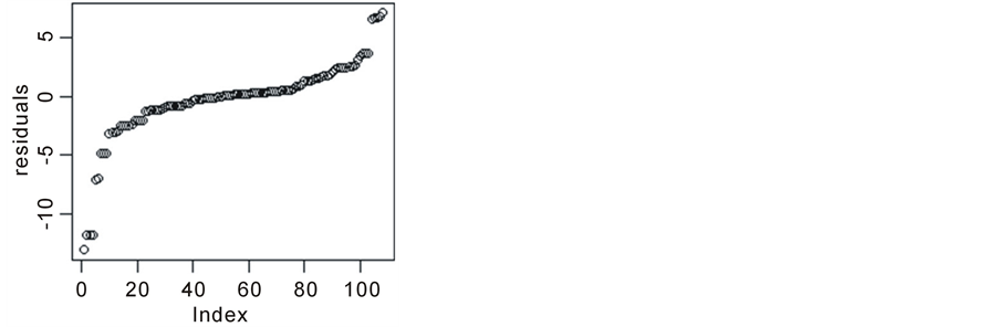
Figure 4. Accumulation of validation errors around 0%.
estimated. It should not be used for order statistics, such as the median, since the y*j would then always take one of two or three values. (The jackknife estimates are degraded if the data set has excessively straggling tails, i.e. a few wild outliers) [31] .
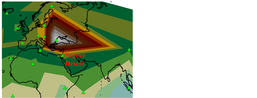
Figure 5 shows a sample of using this method in our processes. Figure 5(a) shows a TIN model generated upon values of all sites in year 2010. Figure 5(b) is the same model but by eliminating the Negev Desert site. The differences between these two models at the Negev Desert site location may be considered as the amount of gas absorption or emission in that region in the year 2010.
In this sample the (Figure 5(b)) TIN model illustrates that if no gas emission or absorption had been occurred in the Negev Desert region, the existence of CO2 gas in that place might be 401.97 Pg∙C∙yr−1. This is while the observed amount for this site in 2010 indicates existence of 391.83 Pg∙C∙yr−1 of gas, which is 10.14 units less than expected amount. So it may be true to suppose that Negev Desert region has contained a gas sink factor by the amount of 10.14 units in the year 2010, although its related measurement site, shows existence of massive amount of gas in that period of time. By continuing this process for each of sites in each year and considering the results and trends of them, it will be possible to extract out the most absorption or emission places among them all.
4. Results
4.1. Main TIN models
As described previously, for each of the years between 2000 and 2011, a TIN model has been generated based on the data of all related sites. These models were cited in this study as a basis for observation of CO2 in each point of the Globe for those years. As it can be seen in Figure 6, the value of the highest amount of gas has been grown from 377.85 Pg∙C∙yr−1 in 2000 to 407.44 in 2011, and likewise, the value of the lowest amount of the gas grew from 366.24 Pg∙C∙yr−1 in 2000 to 386.73 in 2011, which indicate the growth of Global gas balance by passing time. In a glance it indicates that in all the years, the Black Sea region represents the largest inventory of gas, and consequently there should most probably be a strong and permanent factor of gas emission over there. Another apparent conclusion that can be drived from Figure 6 is that the accumulation of gas in the Southern Hemisphere is less than its Northern counterparts.
To find out more analytical deductions from these elegant data, we applied “Leave One Out” processes over them and generated one special pseudo-TIN model for each one of sites in each year, based on eliminating them, and comparing their subsequent outgrowth with their actual observations. This will be more elaborated in the next section.
4.2. Leave One Out Pseudo-Values
Applying “Leave One Out” method to the explained data, the pseudo-values for each site extracted from them, will represent their actual regional emission or absorption effects. To determine the regional extent of each site, we used “Thiessen polygons” method. In 1911 the climatologist A. H. Thiessen suggested a new method of representing precipitation data from unevenly distributed weather stations. He defined regions based on a set of
 (a)
(a) (b)
(b)
Figure 5. Sample of spatial implementation of “Leave One Out” method. (a) Excerpt of the TIN model generated upon the values of all sites in the year 2010; (b) Same as a but eliminating the Negev Desert site.
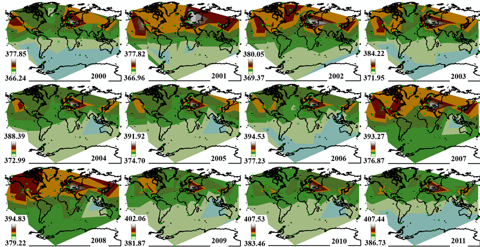
Figure 6. The main TIN models for the years between 2000 and 2011. In this study each of these was used for estimating the gas amount at any point of the planet within those years.
data points in the plane (weather stations) such that “regions be enclosed by a line midway between the station under consideration and surrounding stations” [32] . Based on this proposal the term Thiessen polygon has since been commonly used in geography to denote polygons defined by proximity criteria with respect to a set of points in the plane [33] . Thiessen diagram is a way of dividing space into a number of regions. A set of points (called seeds, sites, or generators) is specified beforehand and for each seed there will be a corresponding region consisting of all points closer to that seed than to any other. Figure 7 shows our results for most absorption and emission activities during the years 2000 to 2011. As it is observable, in 8 out of 12 years, there exist one most absorption activity for every most emission activity. This confirms that the absorption rate also rises with increased emission rate, but with lower proportion.
By applying the proposed method to data of CO2 measuring stations during the years 2000 to 2011, the degree of each station activity in each year were calculated and stored. Table 1 shows 10 stations that have the highest degree of positive and negative CO2 activities. Each year of 2009 and 2011 contain two of most high absorption
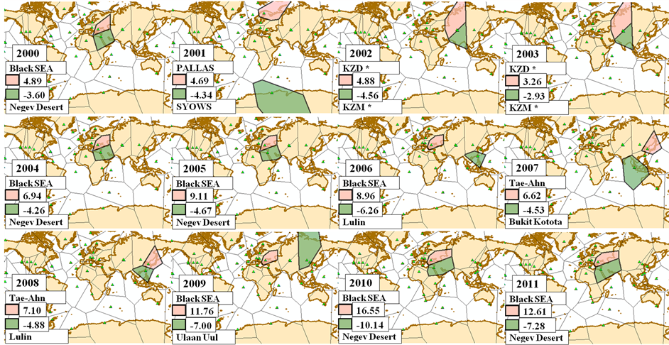
Figure 7. The spots of most emission and absorption for the years between 2000 and 2011, based on “Leave One Out” processes. Interesting subjects may be those which two extremes are adjacent to each other.

Table 1. Ten high impacts among all the amount of carbon dioxide between 2000 and 2011.
activities.
It is obvious that the station “Black Sea” is a more prominent and dominant emission place than all other ones. This station was in all first places of five categories accounted for the highest activities and can be used as an option for the location of the CO2 emission source. Former researches have confirmed huge amount of gas emission in BSC site location [34] . In the Black Sea, measurements were performed on R/V Professor Vodyanitsky during the two CRIMEA cruises, May-June 2003 and 2004. In the north western Black Sea, hundreds of active gas seeps were detected along the shelf and slope of the Crimea Peninsula at water depths between 35 and 800 m. Active gas seeps down to 2100 m water column were also detected. These transport mechanisms allow us to estimate the conditions and means by which gas released from seeps reaches the surface. In dispersed seeps, which typically occur at the shallow sites, gas is released intermittently as bubbles. Vertical transport is therefore by bubble dissolution in the water column, or gaseous release to the atmosphere. The model, which includes argon, nitrogen, oxygen, methane and CO2, was verified using air bubbles in shallow conditions.
On the opposite side according to table1 amounts, the station (WIS) at Negev Desert seems to be as a place with high potential of absorbing gas. By observing the physical locations of both the BSC and WIS stations, it can be seen that the vicinity of poor gas adsorption (WIS) with a strong regional emissions (BSC), caused it to be misdiagnosis. In all the years that have been mentioned in table1, the WIS station values were among the 15 most high amounts, which shows large inventory of gas. However, Leave One Out method indicated that there existed about 391.83 Pg∙C∙yr−1 of gas in the year 2010 in Negev Desert. If no absorption had been taken place over there in that period of time, there might have been 401.97 Pg∙C∙yr−1 gas, due to existence of 407.55 Pg∙C∙yr−1 CO2 over its neighbor at Black Sea site. Researches show that the plants in desert arid lands which have high density of CO2 gas in atmosphere may act as high sequester of atmosphere CO2 [35] . Possible explanations for the high sequestration performance involve the ability of the trees to absorb carbon dioxide without opening pores excessively, which would compromise the tree’s water balance, through evaporation. Presumably, the increased CO2 in the atmosphere makes it easier for trees to efficiently absorb CO2. In addition, the conifers planted are specially selected for their ability to thrive under drought and relatively saline conditions. Yatir forest planted at arid lands of the Negev Desert 40 years ago is expanding at unexpectedly high rates. From this study’s point of view the high amount of CO2 gas emitted from Black sea causes the Yatir forest to grow in an arid land while absorbing higher amount of CO2.
5. Conclusions
The objective of this work has been to show that by using appropriate spatial analysis (in this case “Leave One Out” method), some CO2 sink spots may be extracted out from the amounts of gas inventory in different parts of the Globe. Identifying the places of gas absorption and their ecological characteristics, may lead us to find new factors of gas adsorption. By implementing these absorption factors besides those emission sources which mostly for economic reasons cannot be stopped, we can reduce their environmental impacts. Result of the study has identified that Negev Desert region consists of a strong factor of carbon dioxide absorption. The main ecological characteristic of that location is the growth of Yatir forest in such arid land. Studies have conceived researchers that the trees which are planted in dry and arid deserts may begin to grow and develop if the concentration of CO2 in their atmosphere is high enough.
According to this study, the required carbon dioxide for planted Yatir forest in arid Negev Desert has been provided through its neighborhood by the high quantity of CO2 gas released from the Black Sea region.
Therefore it could be possible to plant a band of suitable trees around the center of a CO2 diffuser with no need of irrigation and at the same time reduce the excessive carbon dioxide in the atmosphere.
Acknowledgements
We wish to thank Dr. Babak Naimi for his informative classes which provided us the validation techniques which were used in this study.
References
- Shim, C., Lee J. and Wang Y. (2013) Effect of Continental Sources and Sinks on the Seasonal and Latitudinal Gradient of Atmospheric Carbon Dioxide over East Asia. Atmospheric Environment, 79, 853-860. http://dx.doi.org/10.1016/j.atmosenv.2013.07.055
- Schonwiese, C.-D., Houghton, J.T., Meira Filho, L.G., Callander, B.A., Harris, N., Kattenberg, A. and Maskell, K. (Eds.) (1997) Climate Change 1995, The Science of Climate Change. Journal of Atmospheric Chemistry, 27, 105-106. http://dx.doi.org/10.1023/A:1005850912627
- Middelkoop, H., Daamen, K., Gellens, D., Grabs, W., Kwadijk, J.C.J., Lang, H., Parmet, B.W.A.H., Schodler, B., Schulla, J. and Wilke, K. (2001) Impact of Climate Change on Hydrological Regimes and Water Resources Management in the Rhine Basin. Climatic Change, 49, 105-128. http://dx.doi.org/10.1023/A:1010784727448
- Heidersbach, T., et al. (2012) Climate Action Plan Technical Report.
- Grewe, V., Dahlmanna, K., Matthesa, S. and Steinbrechtb, W. (2012) Attributing Ozone to NO < sub> x Emissions: Implications for Climate Mitigation Measures. Atmospheric Environment, 59, 102-107. http://dx.doi.org/10.1016/j.atmosenv.2012.05.002
- Sarmiento, J.L., Wofsy, S.C. and Us, A. (1999) Carbon Cycle Science Plan.
- Kuang, Z., et al. (2002) Spaceborne Measurements of Atmospheric CO2 by High-Resolution NIR Spectrometry of Reflected Sunlight: An Introductory Study. Geophysical Research Letters, 29, 11-1-11-4.
- Ciais, P., et al. (1995) A Large Northern Hemisphere Terrestrial CO2 Sink Indicated by the 13C/12C Ratio of Atmospheric CO2. Science, New York, Washington, 1098-1098.
- Tans, P.P., Fung, I.Y. and Takahashi, T. (1990) Observational Constraints on the Global Atmospheric CO2 Budget.
- Le Quéré, C., Raupach, M.R., Canadell, J.G., Marland, G., et al. (2009) Trends in the Sources and Sinks of Carbon Dioxide. Nature Geoscience, 2, 831-836. http://dx.doi.org/10.1038/ngeo689
- Canadell, J.G., Le Quéré, C., Raupach, M.R., Field, C.B., Buitenhuis, E.T., Ciais, P., Conway, T.J., Gillett, N.P., Houghton, R.A. and Marland, G. (2007) Contributions to Accelerating Atmospheric CO2 Growth from Economic Activity, Carbon Intensity, and Efficiency of Natural Sinks. Proceedings of the National Academy of Sciences of the United States of America, 104, 18866-18870. http://dx.doi.org/10.1073/pnas.0702737104
- Susan, S. (2007) Climate Change 2007. The Physical Science Basis: Working Group I Contribution to the Fourth Assessment Report of the IPCC, Vol. 4. Cambridge University Press, Cambridge.
- Conway, T.J., Raatz, W.E. and Richard, H.G. (1985) Airborne CO2 Measurements in the Arctic during Spring 1983. Atmospheric Environment (1967), 19, 2195-2201. http://dx.doi.org/10.1016/0004-6981(85)90128-3
- Assonov, S.S., Brenninkmeijer, C.A.M., Schuck, T. and Umezawa, T. (2013) N2O as a Tracer of Mixing Stratospheric and Tropospheric Air Based on CARIBIC Data with Applications for CO2. Atmospheric Environment, 79, 769-779. http://dx.doi.org/10.1016/j.atmosenv.2013.07.035
- Longinelli, A., Langone, L., Ori, C. and Selmo, E. (2011) Atmospheric CO2 Concentrations and δ13C over Western and Eastern Mediterranean Basins during Summer 2007. Atmospheric Environment, 45, 5514-5522. http://dx.doi.org/10.1016/j.atmosenv.2011.06.024
- Nassar, R., Jones, D.B.A., Kulawik, S.S., Worden, J.R., Bowman, K.W., Andres, R.J., et al. (2011) Inverse Modeling of CO2 Sources and Sinks Using Satellite Observations of CO2 from TES and Surface Flask Measurements. Atmospheric Chemistry and Physics, 11, 6029-6047. http://dx.doi.org/10.5194/acp-11-6029-2011
- NOAA (2011) CCGG Measurement Sites. http://www.esrl.noaa.gov/gmd/ccgg/tables/?columns=code% 7Cname%7Ccountry%7Clat%7Clon%7Calt%7Ccoop_name&table_type=active&project=all¶m=CO& pos_label=decimal
- CO2/Flask. FTP Directory (2011) /data/trace_gases/co2/flask/ at aftp.cmdl.noaa.gov. ftp://aftp.cmdl.noaa.gov/data/trace_gases/co2/flask/
- Fan, S., Gloor, M., Mahlman, J., Pacala, S., Sarmiento, J., Takahashi, T. and Tans, P. (1998) A Large Terrestrial Carbon Sink in North America Implied by Atmospheric and Oceanic Carbon Dioxide Data and Models. Science, 282, 442-446. http://dx.doi.org/10.1126/science.282.5388.442
- Legendre, P. (1993) Spatial Autocorrelation: Trouble or New Paradigm? Ecology, 74, 1659-1673. http://dx.doi.org/10.2307/1939924
- Fortin, M.J., Dale, M.R. and Hoef, J. (2006) Spatial Analysis in Ecology. Encyclopedia of Environmetrics.
- Peucker, T.K., et al. (1978) The Triangulated Irregular Network. In: American Society of Photogrammetry, Digital Terrain Models Symposium, St. Louis, Missouri, 9-11 May 1978, 532.
- Abdi, H. and Williams, L. (2010) Encyclopedia of Research Design. Jackknife, I.N.S., Ed., Sage, Thousand Oaks.
- Martinez, N.T., Horvitz, C., Erickson, K. and Palmer, M.I. (2013) Spatial Distributions of Native and Invasive Shrubs in a Sub-Tropical Forest.
- Griffith, D.A. (1987) Spatial Autocorrelation. Association of American Geographers, Washington DC.
- Dormann, C.F., McPherson, J.M., Araújo, M.B., Bivand, R., Bolliger, J., Carl, G., et al. (2007) Methods to Account for Spatial Autocorrelation in the Analysis of Species Distributional Data: A Review. Ecography, 30, 609-628. http://dx.doi.org/10.1111/j.2007.0906-7590.05171.x
- Naimi, B., Skidmore, A.K., Groen, T.A. and Hamm, N.A.S. (2011) Spatial Autocorrelation in Predictors Reduces the Impact of Positional Uncertainty in Occurrence Data on Species Distribution Modelling. Journal of Biogeography, 38, 1497-1509. http://dx.doi.org/10.1111/j.1365-2699.2011.02523.x
- De Jong, P., Sprenger, C. and Veen, F. (1984) On Extreme Values of Moran’s I and Geary’s c. Geographical Analysis, 16, 17-24. http://dx.doi.org/10.1111/j.1538-4632.1984.tb00797.x
- Joseph, V.R., Hung, Y. and Sudjianto, A. (2008) Blind Kriging: A New Method for Developing Metamodels. Journal of Mechanical Design, 130, Article ID: 031102. http://dx.doi.org/10.1115/1.2829873
- Xiong, Y., Chen, W., Apley, D. and Ding, X.R. (2007) A Non-Stationary Covariance-Based Kriging Method for Metamodelling in Engineering Design. International Journal for Numerical Methods in Engineering, 71, 733-756. http://dx.doi.org/10.1002/nme.1969
- Hanna, S.R. (1989) Confidence Limits for Air Quality Model Evaluations, as Estimated by Bootstrap and Jackknife Resampling Methods. Atmospheric Environment (1967), 23, 1385-1398. http://dx.doi.org/10.1016/0004-6981(89)90161-3
- Thiessen, A.H. (1911) Precipitation Averages for Large Areas. Monthly Weather Review, 39, 1082-1089.
- Brassel, K.E. and Reif, D. (1979) A Procedure to Generate Thiessen Polygons. Geographical Analysis, 11, 289-303. http://dx.doi.org/10.1111/j.1538-4632.1979.tb00695.x
- McGinnis, D. (2005) Vertical Pathways of Methane in the Black Sea. Geophysical Research Abstracts, 7, Article ID: 00077.
- Tal, A. and Gurion, B. (2009) Making Forestry Sustainable: Recent Israeli Innovations in Eucalyptus Farming and Carbon Sequestration. In: Seeing the Forest beyond the Trees, Proceedings of the 2009 IUFRO 3.08 Small-Scale Forestry Symposium, Morgantown, West Virginia, 7-11 June 2009, 237-244.
NOTES

*Corresponding author.