Journal of Geographic Information System
Vol.5 No.6(2013), Article ID:40630,13 pages DOI:10.4236/jgis.2013.56050
GIS-Based Local Spatial Statistical Model of Cholera Occurrence: Using Geographically Weighted Regression
Department of Geography and Regional Planning, University of Benin, Benin City, Nigeria
Email: *nkekifndidi@gmail.com
Copyright © 2013 Felix Ndidi Nkeki, Animam Beecroft Osirike. This is an open access article distributed under the Creative Commons Attribution License, which permits unrestricted use, distribution, and reproduction in any medium, provided the original work is properly cited.
Received October 24, 2013; revised November 24, 2013; accepted December 1, 2013
Keywords: Local Statistics; Global Statistics; Geographically Weighted Regression; Cholera; Ordinary Least Square
ABSTRACT
Global statistical techniques often assume homogeneity of relationships between dependent variable and predictors across space. This assumption has been criticized by statistical geographers as a fundamental weakness that may yield misleading result when it is applied to dataset with spatial context. To strengthen this weakness, a new method that accounts for heterogeneity in relationships across geographic space has been presented. This is one of the family of local spatial statistical techniques referred to as geographically weighted regression (GWR). The method captures non-stationarity of relationship in spatial data that the ordinary least square (OLS) regression fails to account for. Thus, the paper is designed to explore and analyze the spatial relationships between cholera occurrence and household sources of water supply using GIS-based GWR, also to compare the modeling fitness of OLS and GWR. Vector dataset (spatial) of the study region by state levels and statistical data (non-spatial) on cholera cases, household sources of water supply and population data were used in this exploratory analysis. The result shows that GWR is a significant improvement on the global model. Comparing both models with the AICc value and the R2 value revealed that for the former, the value is reduced from 698.7 (for OLS model) to 691.5 (for GWR model). For the latter, OLS explained 66.4 percent while GWR explained 86.7 percent. This implies that local model’s fitness is higher than global model. In addition, the empirical analysis revealed that cholera occurrence in the study region is significantly associated with household sources of water supply. This relationship, as detected by GWR, largely varies across the region.
1. Introduction
The “one model fits all” syndrome that characterized global statistical techniques has motivated modern geographers and other spatial analysts to model and explore the local pattern of relationships that exist between variables. The global techniques such as regression (which is the widely used method of estimating relationships in the social science) often assumed a generalized pattern of association across the studied space. When applied to spatial data, it is quick to assume a constant relationship over space with respect to the processes being examined. The fact remains that it has shown that every phenomenon is related to every other phenomenon in space but near (localized) phenomena are more related than distant (global) ones (Tobler’s first law of geography). This fundamental weakness connected with the global method of accessing relationships and spatial association, has stemmed the advancement and development of strings of local spatial statistical models.
These local spatial statistical models, often referred to as disaggregate statistics, are designed to capture both spatial association and diversity (heterogeneity) simultaneously. A comprehensive distinction between global and local statistics can be found in the work of [1] Fotheringham et al., (2002). They described local statistics, on one hand, as a spatial disaggregation of global statistic, which is computed at the individual level and yield multi-valued result. On the other hand, global statistics is the overall average values of a data set which is assumed to represent the situation in every part of the study region and often yields a single-valued result. Following their classical counterpart, contemporary geographers now recognized that every location has an intrinsic degree of distinctiveness even from the closest location in a spatial component or system.
However, the most prominent disaggregate spatial statistical techniques available for empirical analysis, include geographically weighted regression originally designed by [1] Fotheringham et al., (2002); local indicator of spatial association ([2] Anselin, 1995); local Gi* Statistics ([3] Getis and Ord, 1992); local chi-square ([4] Rogerson, 1999); local Moran’s I ([5] Anselin, 1996) and ([6] the variogram cloud plot (Haslett et al., 1991). Basically, the use of these local spatial statistics has become widespread and prominent especially among spatial analysts, geographers, medical practitioners, physical and social scientists. This is because it is fast becoming an established fact that global statistics can no longer satisfy contemporary policy needs.
Empirical literature has shown that the underlying assumption of global statistics is to depict that the relationships between the predictor(s) and the criterion variable are homogenous across space i.e., the same factor initiates the same response in all aspects of the study territory ([7] Mathews and Yang, 2012). In the real world scenario, this may not be the case. The relationships between variables might reveal strong evidence of heterogeneity and vary geographically. Spatial heterogeneity occurs when the same factor provokes a completely different response in different aspects of the study area ([7] Mathews and Yang, 2012).
The global modeling techniques, such as the ordinary least squares regression (OLS), linear and other nonlinear models cannot detect spatial variation and relationships within geographic entities. As a result, intrinsic relationships may be obscured and spatial association between variables in a region is concealed. Such incomplete information (derived from global statistics), when adopted for addressing policy issues, may be counterproductive. To strengthen this weakness, statistical geographers ([8] Brunsdon et al., 1996 and [1] Fotheringham et al., 2002) recently came up with geographically weighted regression (GWR)—a technique designed to explore spatial non-stationarity or heterogeneity in geographic dataset. Spatial non-stationarity is a scenario in which global statistical models cannot explain the relationship between sets of variables ([8] Brunsdon et al., 1996).
GWR presents a platform for exploring the relationships that exist between explanatory variables and the criterion variable across space and such analysis is conducted within a single framework. It is a data exploratory technique carried out in one platform but yields multiple results and explanations. Fundamentally, the result of the analysis can be visualized on a series of maps. Every mapping unit produces its own unique explained value, coefficient and residual. The recent integration of GWR into ESRI ArcGIS has further increased the quality of output. For example, GIS-based GWR has the capability of spatially displaying the parameter estimates and coefficient of determination regarding all variables in a raster surface and vector map respectively for easy and quick visual interpretation of relationships and detected spatial patterns.
Due to its ability to integrate with GIS, by presenting mappable values, the technique has been embraced by researchers and scholars in numerous academic fields. Literature has shown that GIS-based GWR has been applied enormously in the public health and epidemiological-based studies ([9] Lin and Wen, 2011; [10] Nakaya et al., 2005; [11] Yang et al., 2009; [12] Chen et al., 2010 and [13] Goovaerts, 2005). Other areas of application include, environmental and ecological management, monitoring and hazard ([14] Zhang et al., 2004; [15] Fernandez et al., 2013 and [16] Mennis and Jordan, 2005), public policy ([17] Malczewski and Poetz, 2005; [18] Yu et al., 2007; [19] Zhao et al., 2005; [20] Partridge and Rickman, 2005).
The major objectives of this paper are to explore and analyze the spatial relationships that exist between cholera occurrence and household sources of water supply using GIS-based GWR, and to compare the modeling results of the OLS and GWR with respect to the best fit. Using disaggregate statistic to test and model such relationship is a rich and viable methodology for the study of cholera as it is associated with household water supply. It allows the pattern of association to be visualized on a map and all statistical values to be spatially represented on raster maps. Overall, GWR will allow the local parameter estimate and local t-value of the model to be interpolated by allowing the audience to explicitly focus on the main matter of interest. This is possible because it combines the geo-visualization power of GIS to generate its output.
2. Study Region and Data
The data for this empirical analysis were collected from the 36 states (and the Federal capital territory) of Nigeria which is located geographically in West Africa sub-region between latitude 4˚9'N to 13˚46'N and longitude 3˚15'E to 16˚54'E (Figure 1). It has a territorial coverage of about 923,770 km2 inhabited by over 140 million people which make it one of the most populous country in Africa. Like other developing countries, Nigeria is plagued by polio, malaria, sleeping sickness and periodic outbreak of cholera. Cholera pandemic in the country is attributed to the poor quality of health care and inadequate access to potable water.
The first cholera outbreak in Nigeria occurred in 1970 (in a Town near Lagos) leading to case fatality rate (CFR) of 12.8 percent. Between then and the end of 1990 few
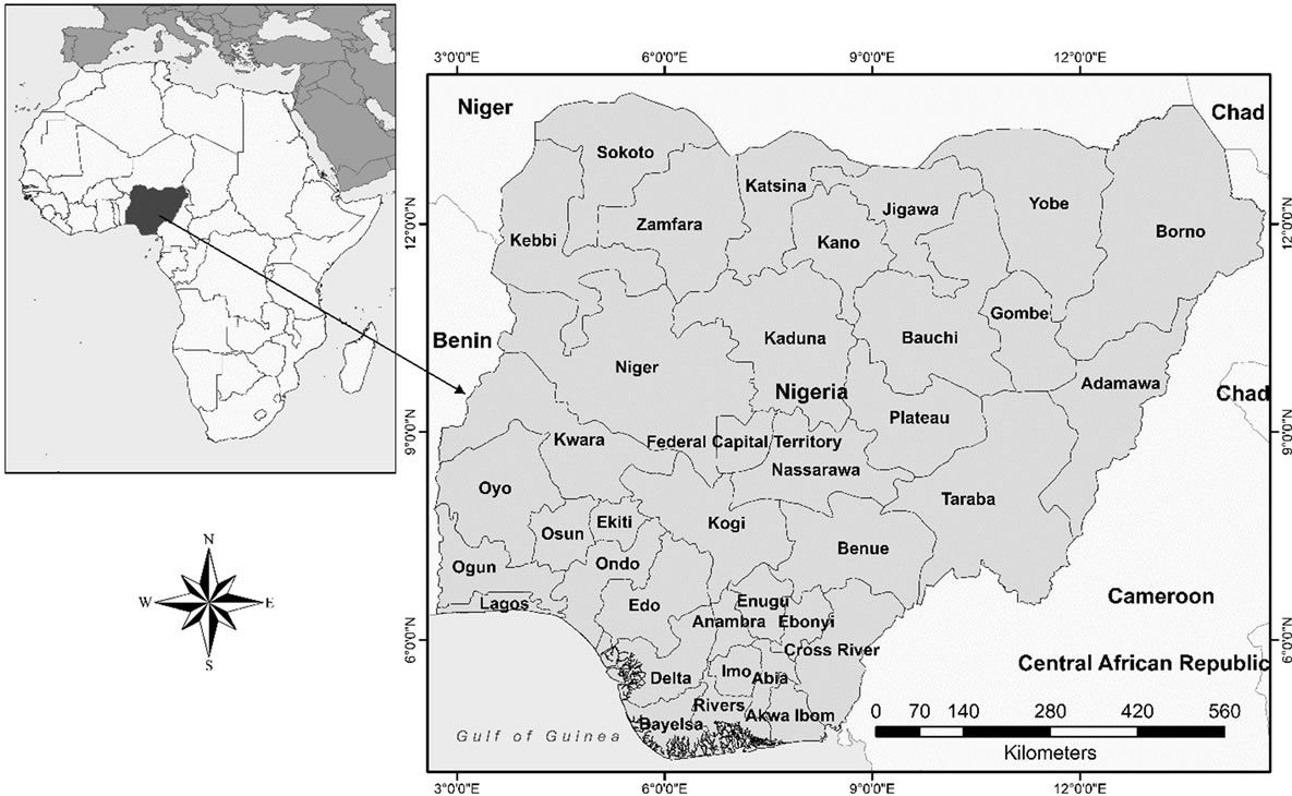
Figure 1. Location of the study region-the 36 states and Federal capital territory (FCT).
cases were reported. In 1991, another outbreak occurred with CFR of 12.9 percent (this marks the highest for the country up to 2012). Since then, it has dropped to between 4.1 and 3.6 percent.
The data used in this empirical analysis are divided into two parts-spatial and non-spatial datasets. The spatial dataset which comprises the vector map of Nigeria (showing the 37 states including FCT) was downloaded from map library database in ESRI shape file format. This was re-projected from geographic coordinate systems (GCS) to projected coordinate systems using the world geodetic system (WGS) 1984 web Mercator. The non-spatial data consist of statistical figures on cholera occurrence and the sources of household water supply. Data on cholera occurrence for 2005 and major sources of household drinking and cooking water for 2005 at state level were used for the analysis and this was collected from the National Bureau of Statistics in the country. To determine and compute population density, the 2006 population census data was obtained from Nigeria Population Commission by state level.
3. Methodology
In this empirical analysis, the basic software used for computation, exploratory analysis, mapping and visualization is ESRI ArcGIS version 10.1. This GIS software was chosen because it presents numerous extensions for spatial statistical and geostatistical modeling (such as OLS, GWR, spatial autocorrelation and other geostatistical analyst tools). Generally, these techniques were used to map spatial pattern, test relationships, check for redundancy among the explanatory variables and geovisualization. The model’s framework is shown in Figure 2. The dependent variable for this model is the documented cholera cases for 2005 by state level. This statistical values were entered into the prepared GIS vector polygon map as non-spatial data. To visualize the spatial distribution of such data, a choropleth map was generated to show the density of cholera occurrence in the country. It was normalized with the area coverage polygons (in km2) by state and a five-class natural breaks (Jenks) classification method was applied (Figure 3(a)). In order to detect cholera hotspots and show continuous distribution, empirical Bayesian kriging model with log empirical data transformation method was applied on the map (Figure 3(b)).
Basically, the first fundamental geographic question (the where question) regarding cholera occurrence in the study region has been answered by Figure 3(b) (i.e. by displaying the location of cholera hotspots and the spatial pattern of distribution). The next logical geographic questions that follow are “why” such clustering pattern? And “what” are the likely factors that are associated with this observed pattern? The GWR is designed to answer such scientific questions and others like, does the rela-
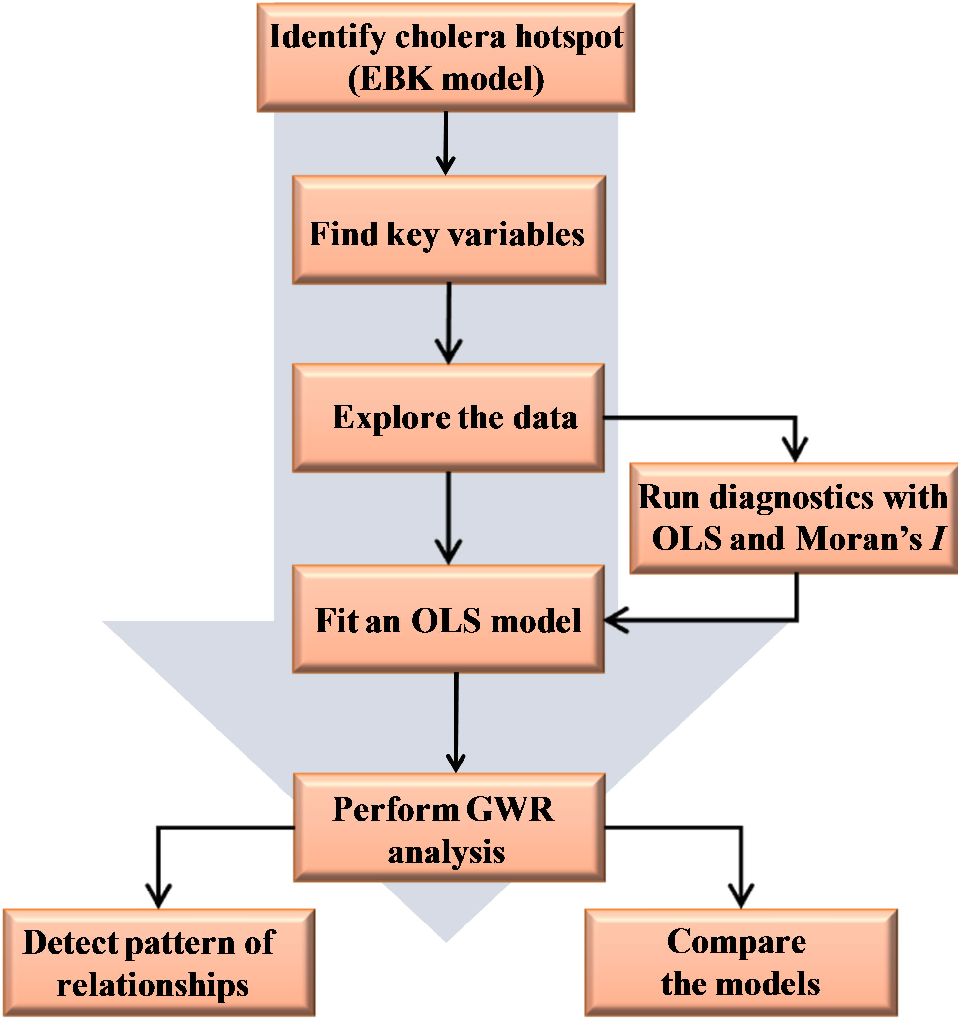
Figure 2. Methodological framework.
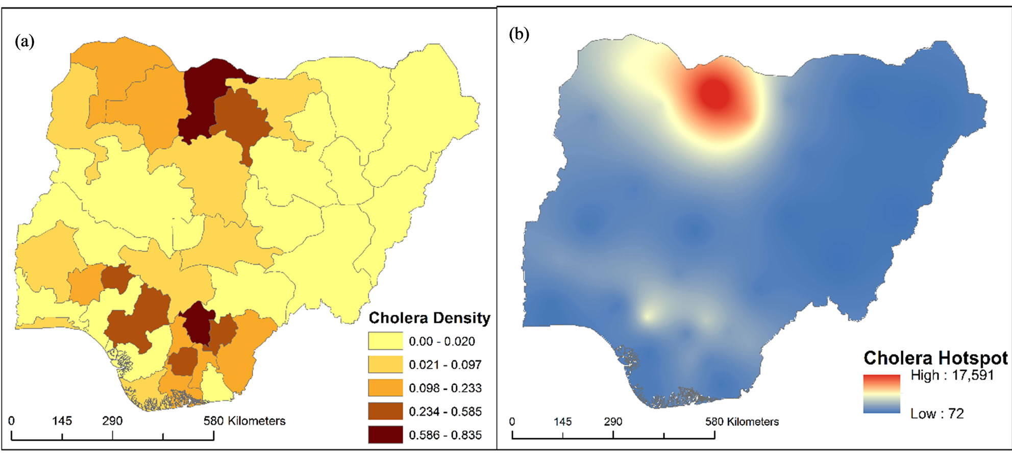
Figure 3. Cholera spatial distribution of Nigeria.
tionship between the dependent variable and the predictors varies across space? Which explanatory variable shows stronger influence in a certain area?
Six major categories of household source of cooking and drinking water were identified and selected for the analysis as explanatory variables. Population density was included as a predictor variable because it may exert strong influence over cholera occurrence and spread (i.e. it is expected that cholera cases would be high in high population density areas). To better understand the spatial pattern of distribution, the seven explanatory variables were visualized with interpolated raster surface (Figure 4). Tanker (variable) represent water vendors either by tanker trucks or water hawkers. Rain and well variable include those that depend on rain water by collecting and storing in a well during the wet season. Pipe borne variable involves the treated source of household water managed by government board. This is distributed to households through underground pipes. Borehole as a source of household water supply is usually untreated and mostly privately owned and in some cases, shared by group of people or communities.
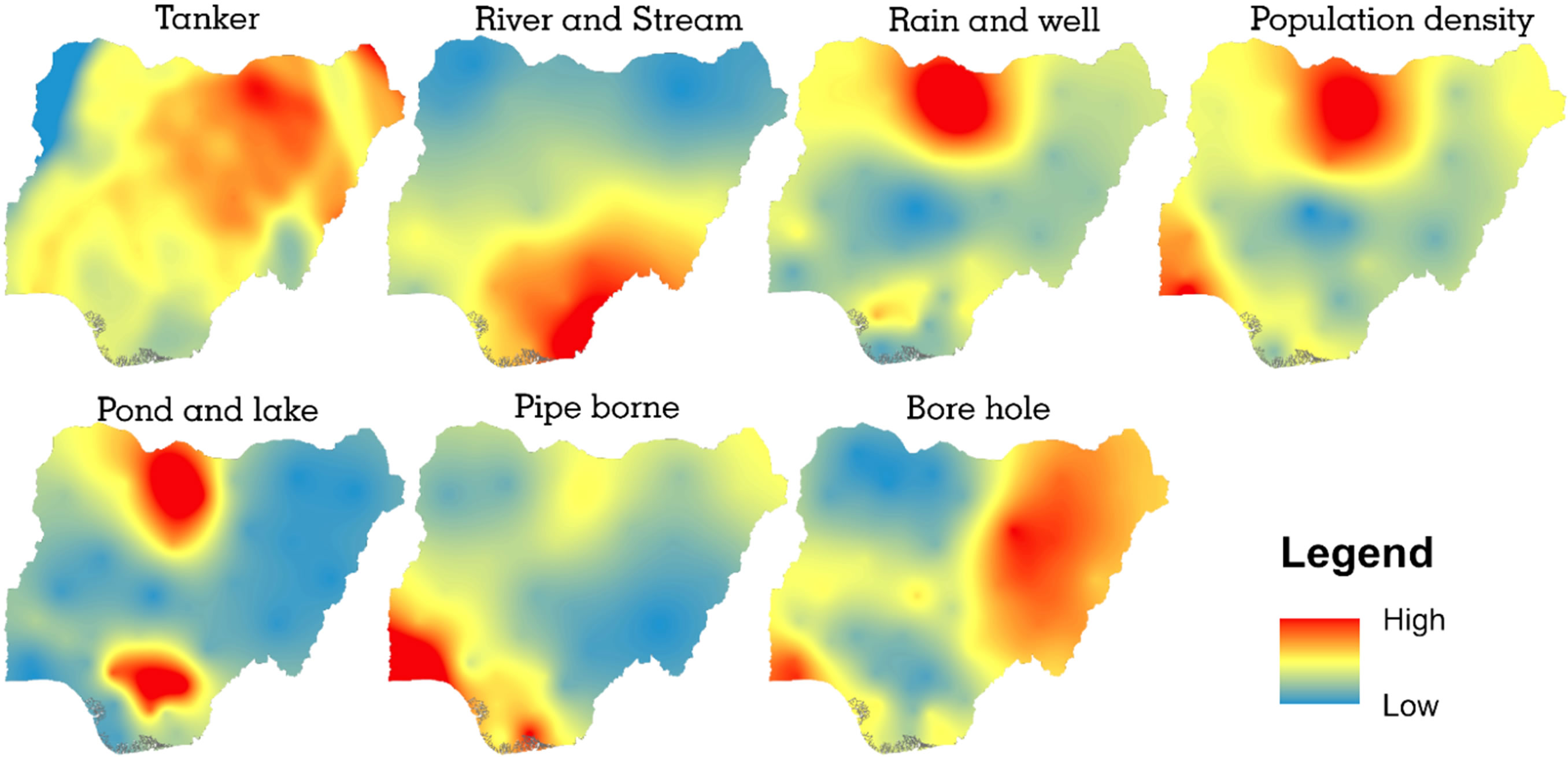
Figure 4. Selected explanatory variables.
Tools for Modeling Spatial Relationships
In this paper, the OLS and GWR spatial statistical tools were employed for exploring the spatial relationships between cholera occurrence and the seven predictors. The OLS was used as a diagnostic tool and for selecting the appropriate predictors (with respect to their strength of correlation with the criterion variable) for the GWR model. It can automatically check for multicollinearity (redundancy among predictors).
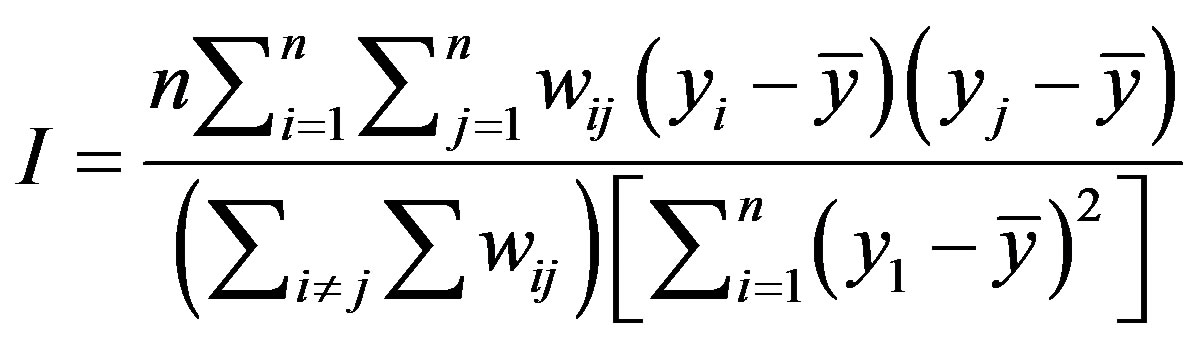
The multicollinearity was assessed with the variance inflation factor (VIF) values of the OLS. If the VIF value(s) is greater than 10, it therefore indicate the existence of multicollinearity among the predictors. In addition, autocorrelation statistic was applied to detect whether there is spatial autocorrelation or clustering of the residuals which violate the assumption of OLS. Progressively, the spatial independency of the residuals was assessed with the global spatial autocorrelation coefficient Moran’s I. This is defined by the equation:
 (1)
(1)
where n represents the total number of states (polygons), i and j depict the various states, yi and yj is the residuals of location i and j respectively,  is the mean of the residual and wij represents a spatial weight matrix for measuring spatial proximity between i and j locations. Moran’s I values ranges from +1 (positive autocorrelation) and −1 (negative autocorrelation). The expected outcome in this case is a complete random pattern i.e. no spatial autocorrelation.
OLS is a global statistical model for testing and examining relationships between variables. It uses single equation to estimate the relationship between the dependent variable and the explanatory variable(s) and assumes stationarity or static relationship across the study region. This method computes a single coefficient (implying that its coefficient is constant over space) and average the result of its model which may not represent every cases. The OLS model’s equation for this analysis is presented as:
 (2)
(2)
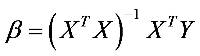
where Y is the criterion variable (cholera occurrence), the betas (β0 to βn) represent the corresponding number of the coefficients of predictors, while X1 to Xn depict the corresponding number of predictors (in Figure 4) and ε is the random error term of the residuals. Assuming that these conditions are satisfied, the OLS parameter estimator is determined as:
 (3)
(3)
where β is the vector of the global model’s parameter to be estimated, X is a matrix of the predictors with elements of first column set to 1, Y represent the vector of the observed values on the dependent variable, and  is the inverse of the variance-covariance matrix.
GWR is a local spatial statistical technique that assumes non-stationarity in relationships. That is the relationships between the dependent variable and the explanatory variable(s) changes from location to locations. GWR on like the global statistics generate an equation for every component in the dataset by calibrating each one using the target feature and its neighbors. In this respect, nearby features produce a higher weight in the calibration than distant features ([21] Scott and Janikas, 2010). This approach may likely uncover spatial relationships or associations neglected by OLS. However, the underlying tenet of GWR is that parameters are likely to be estimated anywhere in the region of study given a criterion variable and one or set of explanatory variables which have been measured in a known location ([22] Charlton and Fotheringham, 2009).
The model multiplies geographically weighted spatial matrix consisting of geo-referenced data. The matrix defines the neighborhood spatial relationships between states and aid the detection of spatial variation in the relationship among the variables. The basic GWR model as developed by [1] Fotheringham et al., (2002) is estimated as:
 (4)
(4)
where  depicts the geographic location (coordinates) of the ith point in space and
  is a realization of the continuous function at point i. That is, continuous surface of parameter values, and measurements of such surface is allowed and is taken at certain points to denote the spatial variability of the surface ([1] Fotheringham et al., 2002).
However, the major output from GWR model for each observation (state) is a set of parameter estimates (local coefficients for each explanatory variable) and associated diagnostics (standard errors, Cook’s D statistics, local R2 statistic, and local standard deviation) that can be visualized within a GIS platform ([22] Charlton and Fotheringham, 2009; [15] Fernandez et al., 2013). The series of maps often generated are vital tools for understanding the level of spatial relationship and show locations were each predictor exhibit stronger influence on the dependent variable.
The GWR model was computed with geographically weighted regression extension in the spatial statistics tool box of ArcGIS 10.1. To allow the automatic specification of appropriate distance or number of nearest neighbors, the adaptive kernel type was used. This allows the spatial context (Gaussian kernel) as a function of feature density to vary in extent. It constructs a smaller spatial context where the feature distribution is dense and larger spatial context where distribution is sparse. In order to determine the optimal bandwidth of the kernel function, the Akaike Information Criterion (AIC) was applied.
4. Results
4.1. Global Model Using OLS
The OLS model was calibrated to diagnose multicollinearity among the explanatory variables and the result shows that the population density variable and tanker variable returned VIF values of 12.812 and 10.416 respectively. Since these values are higher than the set redundancy threshold of 10 the two variables were removed from the model and re-calibrated. Consequently, the R2 value increased from 0.593 to 0.609. The final result of the OLS model is presented in Table 1. However, Table 1 shows that all the predictors returned VIF values fairly greater than 1.0 indicating that none of the variables are redundant. The explanatory variables-bore hole, rain and well, pond and lake returned significant t-values of −1.90, 3.78 and 2.78 respectively.
The OLS global model revealed that it explained about 60 percent (adjusted R2 = 0.60) of the variation in cholera occurrence with AIC = 694.86 (Table 2). The ANOVA returned a significant F-value = 12.22 and the wald statistic has a significant chi-squared value = 30.68. This means that generally, the model prove to be statistically significant. Jarque-Bera statistic returned a non-significant chi-squared value = 3.39 (Table 2) indicating that the model’s prediction is free from bias (i.e. the residuals are normally distributed). The chi-squared value (14.63) of the Koenker statistic is statistically significant. Importantly, it indicates relationship between some or perhaps all of the explanatory variables and the criterion variable are non-stationary or consistent across the region.
The explanation for this is that some independent variables may be important with respect to predicting the outcome of cholera in some states, but in other states may demonstrate weak predictive capability. It is evident that the model’s fitness will likely be improved with GWR (since the Koenker statistic detected non-stationarity in the relationship). This is because GWR assumes that relationships across space are non-static. To investigate the distributive pattern of the residuals, the OLS generated residuals were mapped (Figure 5). A visual examination of the result shows that no pattern exist, instead the model’s residuals exhibit a random noise meaning that there are no clustering of over predictions and under predictions in the model. The poinsettia red
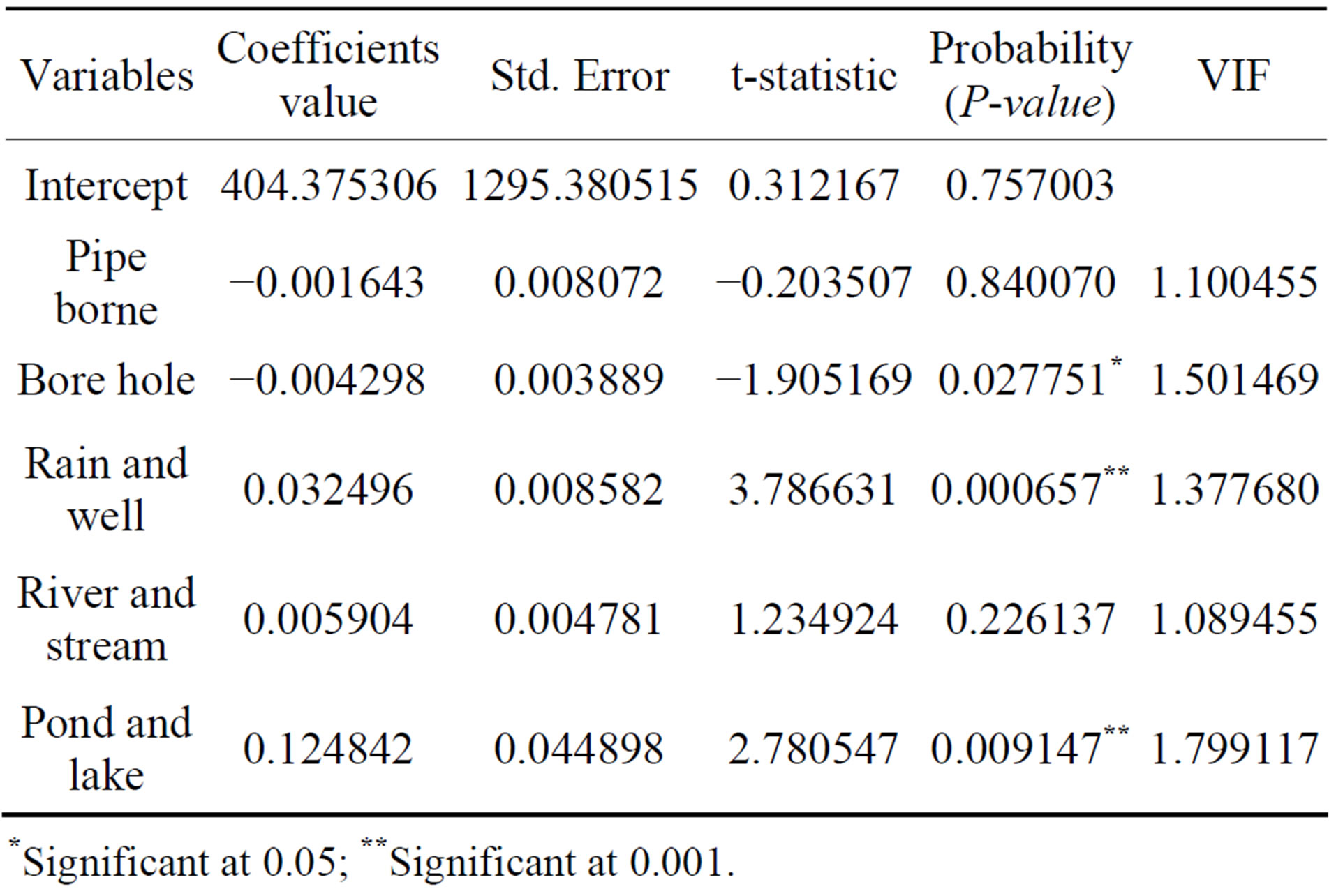
Table 1. Summary of global OLS results.
*Significant at 0.05; **Significant at 0.001.

Table 2. OLS diagnostics statistics.
R2 = 0.663582; Adjusted R2 = 0.609321; AIC = 694.868203; AICc = 698.730272; *Significant parameter at 0.05 level.
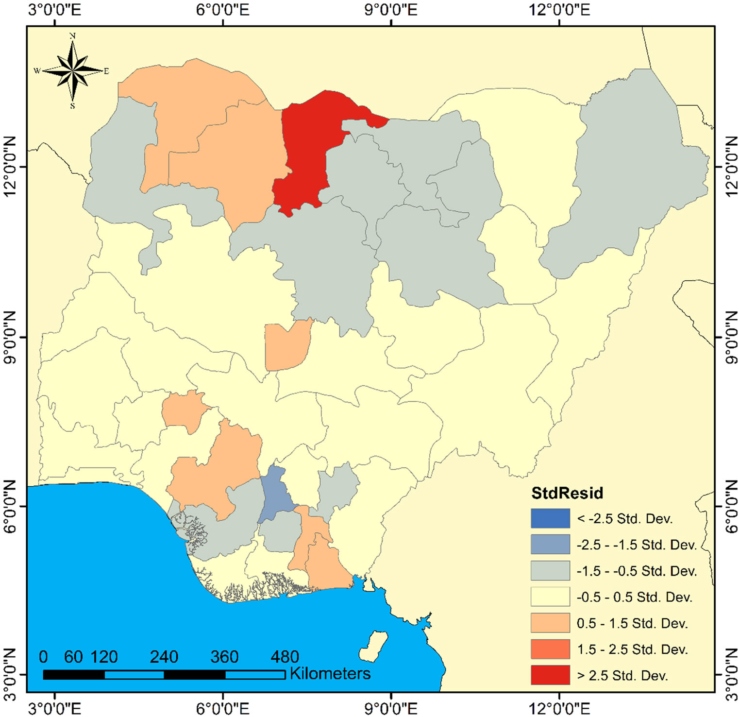
Figure 5. Standardized residuals of the OLS model.
color in Figure 5 depicts the under predicted residuals (positive) while the atlantic blue represents the over predicted (negative residuals).
However, the result was further confirmed statistically by applying spatial autocorrelation statistic (global Moran’s I). This will automatically detect significant clustering or random pattern in the residuals. The Moran’s I report (Figure 6) revealed that the pattern of the residuals is significantly different from random, with a Moran’s index value = −0.05 and z-score value = −0.28. That is the residuals have no statistically significant spatial autocorrelation. In this case, all empirical evidence point to the fact that the OLS residuals fit properly.
4.2. Geographically Weighted Regression
The calibrated GWR results suggest that it is a significant improvement on the global model. Comparing both models with the AICc values, show that the value is reduced from 698.7 (for OLS model) to 691.5 (for GWR model). The difference is roughly 7.2 implying that local models fitness is higher when explaining spatial dataset such as cholera occurrence. As expected, GWR model improved the explaining power of the OLS model with about 10.7 percent (Table 3). This is a high percentage explained value not accounted for by the global model.
Mapping the residuals of GWR indicate that it is randomly distributed (Figure 7). This means the model is properly specified. Verifying with autocorrelation statistic (Moran’s I) returned a randomly distributed residuals with a z-score = −1.14 and Moran index = −0.14.
Figure 8 displays the R2 value as a spatial smoothing of GWR model showing the states where the model’s prediction and strength of relationship is improved. Importantly, that there is regional variation in the strength of relationship in the study region. Overall, the R2 value (0.8) shows a strong significant relationship between cholera occurrence and sources of household water supply. At the regional level, the R2 grouped the states into four sub-regions-those R2 values between 0.8 - 0.7, 0.7 - 0.6, 0.6 - 0.5 and 0.5 - 0.4. In fact, 11 states in the extreme north fall within the first group, 3 and 4 states in the north central fall within the second and third groups respectively while 19 states in the south fall within the last group. The resulting spatial variation in the pattern of

Figure 6. Global Moran’s I spatial autocorrelation.
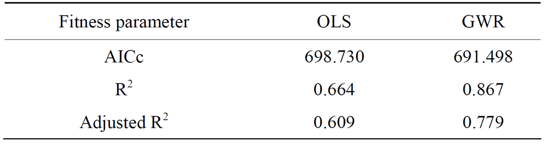
Table 3. Models fitness comparison.
relationships show that the strength of relationship decreases from north to south.
Thus, this pattern suggests local fluctuation in the relationship (non-stationarity). However, the best fit were found in the group of states located in the far north.
A fundamental merit of GWR is its ability to display and visualize the parameter estimate of each explanatory variable on a raster surface. This will make the complex relationship that varies over space easier to comprehend. The resultant surface raster for the predictors show that there is spatial variation in relationship between sources of household water supply and cholera occurrence across the country (Figure 9). Positive and negative relationships were manifested in the result of GWR. The positive relationship means that as the number of household relying on a specific source of water increases, cholera cases equally increases. On the other hand, negative relation-

Figure 7. Standardized residuals for GWR model.
ship implies that as the number of household utilizing a particular source of water increases, cases of cholera reduce. Local coefficient estimate for each explanatory variables are presented in Figure 9. The color ramp is graduated from light to dark gold. Areas with light shade represent areas where that particular variable exhibit strong influence on cholera occurrence while dark shade represent areas where that specific variable exhibit weak or low influence on cholera occurrence.
5. Discussion
Both models (global OLS and local GWR) were able to capture and detect prominent factors (variables) that influence cholera occurrence in the country. However, in this discussion session, only the useful predictors (those without bias that were entered into the local model) will be analyzed. In the exploratory analysis using OLS, five predictors were entered into the models-pipe borne, bore hole, rain and well, river and stream, pond and lake. Pipe borne and bore hole returned negative relationships (Table 1).
The implication of this is that as the number of households utilizing these sources of drinking and cooking water increases, cholera cases decreases. This is not unexpected because these two are the potable (clean and safe) sources of household water supply in the country. Hence, states where majority of its households rely on such sources of water are likely to have lower cases of cholera. Thus, this pattern of relationship can be visually confirmed from Figures 3 and 4. In fact, a cursory examination of cholera hotspot in the former and hotspots for the two predictors (pipe borne and bore hole) in the latter reveals that hotspots of these predictors are found in cholera coldspots.
On the other hand, rain and well, river and stream, pond and lake variables returned positive relationships, implying that cholera cases increase with increasing number of households utilizing these sources of water. This is not uncommon because the spread of cholera disease is often facilitated by unsafe sources of water. Rain and well, river and stream, pond and lake unlike pipe borne and bore hole are open sources that can easily be contaminated.
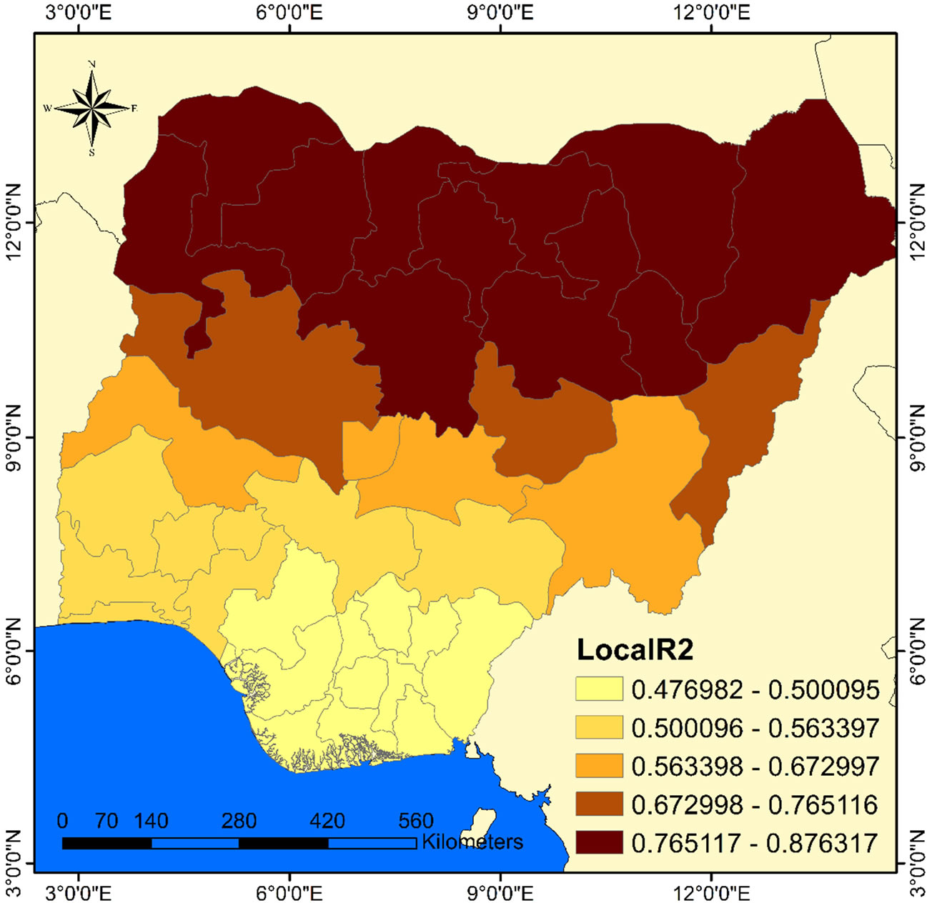
Figure 8. Local R2 smoothing for GWR showing model’s fitness spatial variation.
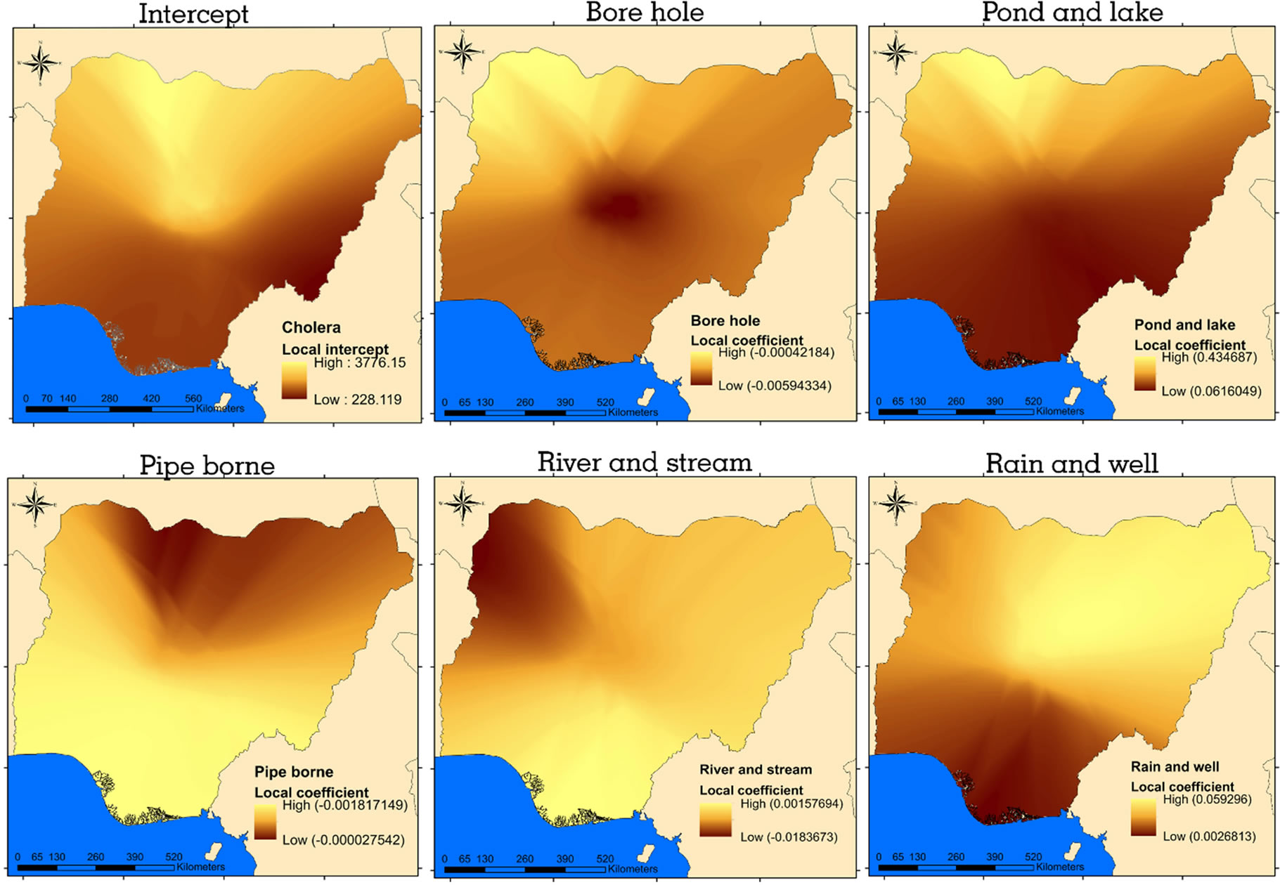
Figure 9. Local parameter estimates of GWR.
Among these 5 explanatory variables, 3 are statistically significant, these are bore hole, rain and well, pond and lake (Table 1). These variables are the most important with respect to explaining cholera occurrence. This result is consistent with the current water situation in Nigeria. Bore hole as a safe source of household water supply is fast becoming the major and recommended source of potable water for domestic use. On the other hand, pipe borne has become unpopular and relegated to certain parts of the country (Figure 4), this is probably the reason while it fails to return significant t-value. This result therefore suggests that bore hole may be an important variable for reducing and checking cholera occurrences.
Rain and well, pond and lake returned a highly significant t-value (i.e. significant at 0.001). Drawing from this, there is 99 percent confidence that cholera occurrence in the study region is positively influenced by these household water sources. A quick visual look at Figures 3 and 4 shows that hotspots for these domestic water sources somewhat overlapped with cholera hotspots. This result is not unexpected because such sources are unsafe and importantly, they are static (unlike river and stream). Thus, they are safe anchorage for breeding, and facilitates the spread of cholera disease.
Generally, OLS model was able to identify three important variables (rain and well, bore hole, pond and lake) that significantly explained the occurrence of cholera in the study region. In the remaining part of this discussion, only these fundamental explanatory variable will be analyzed in detail regarding the local coefficients derived from GWR model. Some predictors exhibited high spatial variability in the resultant parameter estimates of GWR model. In some cases, even contradicted the sign of global parameter estimates of OLS model. These predictors are pipe borne, river and stream, both reflected a combination of negative and positive coefficients across states. Whereas, the OLS global coefficient for pipe borne returned negative value and for river and stream, it returned positive value. This is an evidence that the relationship between the criterion variable and the explanatory variables captured by OLS is more complex and for a reliable result, needs a local model.
As shown by GWR local coefficients, rain and well explanatory variable is an important factor for estimating cholera occurrence. The influence of this predictor is stronger in the north eastern states of the country (Figure 9), this is reasonable because cholera hotspot was detected in this region. While in the south and north-west margin, it is a weak predictor of cholera occurrence. Another important variable is pond and lake, it has high influence in the north western part of the country particularly around the major cholera hotspot. Unlike the former, its sphere of influence is smaller i.e. this variable is a weak predictor of cholera occurrence in majority of the states. This predictor proved to be less relevant in the south central, even though there is high concentration of households that utilize the source water. Ultimately, these two explanatory variables account for significant proportion of cholera occurrence in the northern part of the country, especially the hotspot detected at the north central margin.
Bore hole, as a significant predictor, exhibits strong negative influence over the dependent variable in the north western part of the region. On the central part of the country, the influence is very weak and continued down south-west and south-east. The inverse relationship that bore hole seem to reflect on cholera occurrence especially in the north-west shows that it is a factor not to be over looked with respect to policy making and other epidemiological investigation. As revealed by the local parameter estimates for rain and well, pond and lake variables, that household relying on such sources of water are vulnerable to the disease, bore hole may serve as a factor to lower vulnerability. Especially for the households in the north-west states. The high dependency on bore hole as a source of domestic water supply in the north-east, south-west and central part of the country (Figure 4) is associated with the observed cholera coldspots in these areas (Figure 3). This is confirmed by the local coefficient for bore hole in Figure 9 were the central, north-east and south-west reflects low negative influence on the dependent variable. That is the reason it is not surprising to find high local coefficients values in areas where the variable values are low.
6. Conclusions
This exploratory analysis explains the spatial variation in relationship among geographic dataset and across geographic regions. Using GIS-based local model and global statistic to explore the relationship between cholera occurrences and domestic water supply in Nigeria, it was able to detect and extract certain key information concerning stationarity and non-stationarity in spatial data. Global statistical models often assume homogeneity of relationships between variables across space. This paper has explicitly shown that in spatial data, relationship is not static across geographic space by comparing the results of global OLS and local GWR model’s fitness and parameter estimates.
It was discovered that cholera occurrence in Nigeria is significantly associated with sources of household water supply. Intrinsic among others are rain and well, bore hole, pond and lake. It was found that rain and well, pond and lake sources positively influence cholera occurrence in the region, while bore hole negatively influences it. The observed cholera distribution and clustering pattern are traced to the sources of domestic water supply and this association shows strong spatial heterogeneity across the states.
Finally, this paper is a contribution to the field of GIS, spatial statistics and disease modeling. It presents essential evidence on cholera occurrence in Nigeria and statistically demonstrates that local models exhibit better fitness than global models when modeling spatial data.
REFERENCES
- A. S. Fotheringham, C. Brunsdon and M. E. Charlton, “Geographically Weighted Regression: The Analysis of Spatially Varying Relationships,” Wiley, Chichester, 2002.
- L. Anselin, “Local Indicator of Spatial Association—LISA,” Geographical Analysis, Vol. 27, No. 2, 1995, pp. 93-101. http://dx.doi.org/10.1111/j.1538-4632.1995.tb00338.x
- A. Getis and J. K. Ord, “The Analysis of Spatial Association by Use of Distance Statistics,” Geographical Analysis, Vol. 24, No. 3, 1992, pp. 189-206. http://dx.doi.org/10.1111/j.1538-4632.1992.tb00261.x
- P. A. Rogerson, “Statistical Methods for Geography,” SAGE Publications Ltd, London, 2001.
- L. Anselin, “The Moran Scatter Plot as an ESDA Tool to Assess Local Instability in Spatial Association,” In: M. Fischer, H. Scholten and D. Unwin, Eds., Spatial Analytical Perspectives on GIS in Environmental and SocioEconomic Sciences, 1996, pp. 111-125.
- J. Haslett, R. Bradley, P. Craig, A. Unwin and C. Wills, “Dynamic Graphics for Exploring Spatial Data with Applications to Locating Global and Local Anomalies,” The American Statistician, Vol. 45, No. 3, 1991, pp. 234-242.
- S. A. Mathews and T. C. Yang, “Mapping the Results of Local Statistics: Using Geographically Weighted Regression,” Demographic Research, Vol. 26, No. 6, 2012, pp. 151-166. http://dx.doi.org/10.4054/DemRes.2012.26.6
- C. Brunsdon, A. S. Fotheringham and M. E. Charlton, “Geographically Weighted Regression: A Method for Exploring Spatial Nonstationarity,” Geographical Analysis, Vol. 28, No. 4, 1996, pp. 281-298. http://dx.doi.org/10.1111/j.1538-4632.1996.tb00936.x
- C. Lin and T. Wen, “Using Geographically Weighted Regression (GWR) to Explore Spatial Varying Relationships of Immature Mosquitoes and Human Densities with the Incidence of Dengue,” International Journal of Environmental Research and Public Health, Vol. 8, No. 7, 2011, pp. 2798-2814. http://dx.doi.org/10.3390/ijerph8072798
- T. Nakaya, A. S. Fotheringham, C. Brunsdon and M. Charlton, “Geographically Weighted Poisson Regression for Disease Association Mapping,” Statistics in Medicine, Vol. 24, No. 17, 2005, pp. 2695-2717. http://dx.doi.org/10.1002/sim.2129
- T. C. Yang, P. C. Wu, V. Y. J. Chen and H. J. Su, “Cold Surge: A Sudden and Spatially Varying Threat to Health?” Science of the Total Environment, Vol. 407, No. 10, 2009, pp. 3421-3424. http://dx.doi.org/10.1016/j.scitotenv.2008.12.044
- V. Y. J. Chen, P. C. Wu, T. C. Yang and H. J. Su, “Examining Non-stationary Effects of Social Determinants on Cardiovascular Mortality after Cold Surges in Taiwan,” Science of the Total Environment, Vol. 408, No. 9, 2010, pp. 2042-2049. http://dx.doi.org/10.1016/j.scitotenv.2009.11.044
- P. Goovaerts, “Analysis and Detection of Health Disparities Using Geostatistics and a Space-time Information System: The Case of Prostate Cancer Mortality in the United States, 1970-1994,” Proceedings of GIS Planet, Estoril, 2005.
- L. Zhang, B. Huiquan, C. Pengfei and J. D. Craig, “Modeling Spatial Variation in Tree Diameter-Height Relationships,” Forest Ecology and Management, Vol. 189, No. 1-3, 2004, pp. 317-329. http://dx.doi.org/10.1016/j.foreco.2003.09.004
- J. M. Fernandez, E. Chuvieco and N. Koutsias, “Modelling Long-Term Fire Occurrence Factors in Spain by Accounting for Local Variations with Geographically Weighted Regression,” Natural Hazards and Earth System Sciences, Vol. 13, 2013, pp. 311-327. http://dx.doi.org/10.5194/nhess-13-311-2013
- J. L. Mennis and L. M. Jordan, “The Distribution of Environmental Equity: Exploring Spatial Non-Stationarity in Multivariate Models of Air Toxic Releases,” Annals of the Association of American Geographers, Vol. 95, No. 2, 2005, pp. 249-268. http://dx.doi.org/10.1111/j.1467-8306.2005.00459.x
- J. Malczewski and A. Poetz, “Residential Burglaries and Neighborhood Socioeconomic Context in London, Ontario: Global and Local Regression Analysis,” The Professional Geographer, Vol. 57, No. 4, 2005, pp. 516-529. http://dx.doi.org/10.1111/j.1467-9272.2005.00496.x
- D. L. Yu, Y. D. Wei and C. Wu, “Modeling Spatial Dimensions of Housing Prices in Milwaukee, WI,” Environment and Planning B: Planning and Design, Vol. 34, No. 6, 2007, pp. 1085-1102. http://dx.doi.org/10.1068/b32119
- F, Zhao, L. Chow, M. Li and X. Liu, “A Transit Ridership Model Based on Geographically Weighted Regression and Service Quality Variables,” Final Report Prepared for Public Transit Office, Florida Department of Transportation Lehman Center for Transportation Research, 2005, pp. 1-149. http://lctr.eng.fiu.edu/re-project-link/finaldo97591_bw.pdf
- M. D. Partridge and D. S. Rickman, “Persistent Pockets of Extreme American Poverty: People or Place Based?” Rural Poverty Research Center, Columbia, Working Paper, 2005.
- L. M. Scott and M. V. Janikas, “Spatial Statistics in ArcGIS,” In: M. M. Fischer and A. Getis, Eds., Handbook of Applied Spatial Analysis: Software Tools, Method and Applications, Springer-Verlag, Berlin Heidelberg, 2010, pp. 27-41. http://dx.doi.org/10.1007/978-3-642-03647-7_2
- M. Charlton and A. S. Fotheringham, “Geographically Weighted Regression,” White Paper for Science Foundation, Ireland, 2009, pp. 1-14. http://www.geos.ed.ac.uk/~gisteac/fspat/gwr/arcgis_gwr/GWR_WhitePaper.pdf
NOTES
*Corresponding author.