Journal of Geographic Information System
Vol. 5 No. 3 (2013) , Article ID: 33177 , 10 pages DOI:10.4236/jgis.2013.53019
Integration of Aeromagnetic Data and Landsat Imagery for Structural Analysis Purposes: A Case Study in the Southern Part of Jordan
1Al al-Bayt University, Mafraq, Jordan
2The Hashemite University, Zarqa, Jordan
3University of Jordan, Amman, Jordan
4Natural Resources Authority, Amman, Jordan
Email: *hani1@aabu.edu.jo
Copyright © 2013 Hani Al Amoush et al. This is an open access article distributed under the Creative Commons Attribution License, which permits unrestricted use, distribution, and reproduction in any medium, provided the original work is properly cited.
Received March 24, 2013; revised April 29, 2013; accepted May 29, 2013
Keywords: Landsat TM; Aeromagnetic; Euler Deconvolution; Lineaments; Horizontal Gradients; Analytical Signal
ABSTRACT
In this study, different digital format data sources including aeromagnetic and remotely sensed (Landsat ETM+) data were used for structural and tectonic interpretation of the southern part of Jordan. Aeromagnetic data were analyzed using advanced processing techniques (Spectral analysis, deconvolution). The aeromagnetic interpretation was carried out using the analytical signal, horizontal gradient, vertical gradient, Euler deconvolution. The results were improved by the study of enhanced Landsat ETM+ images and correlated with the extracted surface lineaments. Two main lineament sets are observed in the study area. The major lineaments strike NW-SE, NE-SW and the minor E-W. General coincidence of both landsat and aeromagnetic lineaments trends were observed in the study area, which reflecting the real continuous fractures in the depth. The 3D Euler solution of the study area shows that the depth of the magnetic source body ranges from hundreds of meters to more than 3000 m in the middle northern part of the study area. The combined interpretation of aeromagnetic data and Landsat ETM+, added several significant structural elements, that were previously unrecognized from the separate interpretations of aeromagnetic and remotely sensed data.
1. Introduction
In this study, several digital image-processing techniques were used to enhance the ability of structural interpretation of Landsat ETM+ images. These techniques were integrated with field geophysical exploration using Aeromagnetic Techniques.
Aerial magnetic or aeromagnetic survey applications are very well known in a wide range of geological and exploration studies and they play a very significance role in demarcating the lithological contacts, local and regional geological structures, faults, dykes, lineaments, exploration of mineral ores, hydrocarbon reservoirs and their associated structures, depth to basement, crustal and tectonic studies.
Numerous geophysical studies based on the analysis and processing of potential field have been carried out in south Jordan, e.g. [1] investigated the crustal structures in Jordan using potential field data [2]. Confirmed the sinistral strike-slip motion on the Dead Sea Rift based on aeromagnetic data surveys.
The principle objective of this study is to delineate and mapped the aeromagnetic lineaments and compare them with the surface lineaments deduced from analysis of Landsat Imagery data and surface geological information, demarcate the subsurface faults and depths of magnetic sources bodies. It can also be used to identify the important trends and structures in the magnetic anomaly field.
Landsat ETM+ imageries were downloaded from USGS Global Visualization Viewer website (http://glovis. usgs.gov/). The downloaded images were acquired in August 2003; PCI Geomatics version 9.1 was used for digital image processing and lineaments extraction from the satellite imageries.
The area of study forms the southern part of Jordan Figure 1 with coordinates 13,000E - 270,000E, −140,000N - −63,000N according to Palestine Grid Coordinate system 1924 (PGS). It covers an area of about 11,000 km2. The elevation of study area ranges from 250 m below mean sea level (bmsl) at the most western part of the study area to more than 1800 above mean sea level (amsl) at the eastern and northern parts of the study area. Figure 2 shows the digital elevation model (DEM) for the study area.
2. Geological and Structural Setting
Miocene to recent northward motion of the Arabian plate, which caused the opening of the Red Sea and Gulf of Aden, has controlled much of the fault pattern of Jordan Figure 3. The following fault systems can be noticed in the study area:
1) Ras En-Naqab Fault System (RNFS), which has a NW-SE trend. It most likely has formed as a consequence of extension related to the opening of the Red Sea during the Miocene. Tensional stress evidenced by the NW-SE basaltic dyke intrusions of Ras En-Naqab Fault System has formed an escarpment extending from Ras En-Naqab area in the northwest to Batn Al-Ghul area in the southeast near the Saudi Arabian border with more than 100 km length [3]. This fault zone includes many elongated grabens and horsts in addition to tilted fault blocks in the same trend of the main fault and with variable widths and lengths Figure 3 ([3,4]).
2) Wadi Araba-Dead Sea fault and associated faults. This major fault is distinctive on the Landsat images Figure 2 and extends outside the study area; with a left

Figure 1. Location map of the study area.
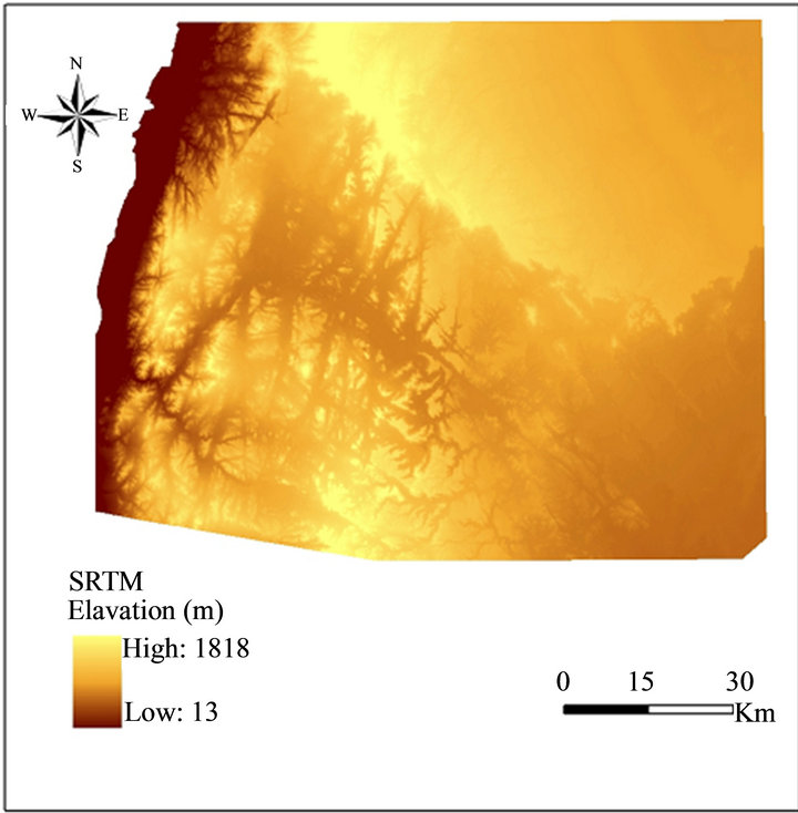
Figure 2. DEM of the study area.
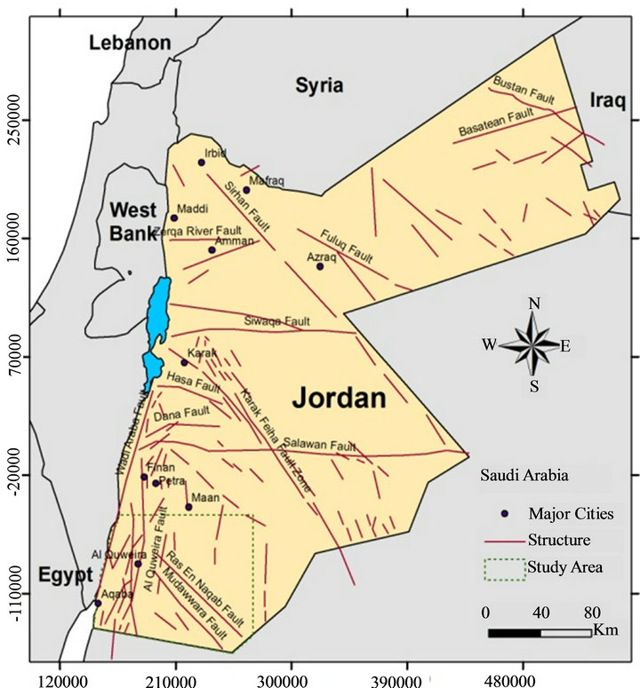
Figure 3. Structural pattern of Jordan (modified [4]).
lateral movement of about 110 km.
3) Al Quweira Fault Zone (QFZ). These faults pass about 4 km west of Petra, (Finan area) and extend for several hundreds of kilometers into Saudi Arabia in the south. These faults are particularly obvious in the AlQuweira area in Jordan Figure 3 [3]. East of the AlQuweira fault zone (QFZ), many N-S faults exhibit sinistral horizontal movement, other faults in south Jordan trend NW-SE and appear to have dip-slip and reverse movements [3]. The displacement along this fault was determined to be 40 km sinistral movement [3]. The study area is characterized by its high diversity in terms of the exposed rock units. Five major types of rock units and formations can be traced; these are Figure 4:
1) The Basement Complex which crops out in the southwestern part of the study area and involves different igneous rock units of Precambrian age. The main rock type is granite (Basement Complex), with varying chemical and mineralogical constituents, such as, granodiorite, basic and acidic intrusive igneous rocks and dolerite. The granite basement is interlaced with many igneous dykes with variable constituents and orientations [5].
2) Disi Sandstone of Paleozoic age, which consist of white to grey cross-bedded sandstone. These rocks were deposited predominantly as large-scale sub-aqueous dunes in high velocity, high discharged braided river with marine incursions [5].
3) Khrayim group of Middle Ordovician-Upper Ordovician age, consisting of silty clay with clay concretion, micaceous fine-grained sandstone with hummocky crossstratification and ripple marks in its lower parts. In the upper part it is composed of highly burrowed micaceous sandstone, thick, massive lensoids of limestone with low angle trough cross-bedding and ripples cross-lamentations inter-bedded with fine-grained sandstone and siltstone. This group covers the most southeastern part of the study area [5].
4) Mesozoic Sandstone, consists mainly of the Lower Cretaceous Kurnub Sandstone Group, this Group rests with a regional angular unconformity on the Ordovician rocks along Ras En-Naqab-Batn Al-Ghoul escarpment. It is characterized by its white-varicolored, fine medium-
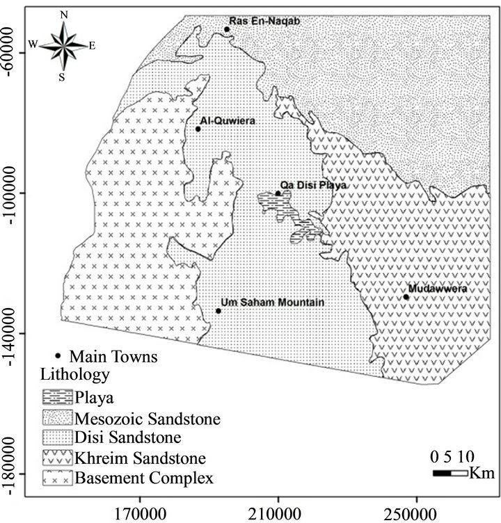
Figure 4. Simplified geological map of the study area [4].
grained, moderate to well sorted cross-bedded sandstone with silty clay and some soil horizons. The depositional environment was predominantly fluvial to marginal marine [5].
5) Volcanic rocks represented by NW-SE trending Miocene-Pliocene basaltic dykes found in the southern part of the study area, locally intruded along the QuweiraMudawwera fault system and containing blocks of Upper Cretaceous limestone and chert [5].
3. Aeromagnetic Study
3.1. Data Sources and Methodology
The aeromagnetic data were provided by the Natural Resources Authority (NRA) in Jordan. They are part from a countrywide airborne magnetic survey which was carried out in 1979-1980 by Geoterrex limited [6]. The data were available in the form of a final dataset corrected for the time-magnetic variations [7]. These data were digitized, plotted and interpolated at a grid points using Surfer Version 8.0, and a total aeromagnetic map was prepared Figure 5. High and low pass filtering techniques were applied on the dataset for enhancement and removing undesired signals. The total aeromagnetic intensity datasets were incorporated into ArcGIS 9.3 environment for further subsequent analysis.
3.1.1. Total Aeromagnetic Intensity Map
The total magnetic field, scale 1:500,000 in the study area Figure 5 ranges from 42,700 to 43,570 nT. It shows two large dominant magnetic anomalies. The first is elongated feature with NE-SW orientation located in the western part of the study area, having a strike 015 - 030
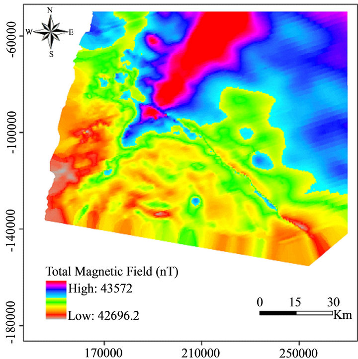
Figure 5. Total magnetic field map.
degrees, and a length of more 110 km. It was interpreted as a major fault because its boundaries are sharply terminated, and it is coincides with the Quwiera fault. The second large magnetic anomaly is a NW-SE elongated feature, having a strike of about 110 - 130 degrees, and a length is more than 100 Km, and is associated with the Ras En-Naqab escarpment and Mudawwara Fault. The aeromagnetic intensity map clearly reflects the underlying basic geology of the study area. The basement that crop out in the study area produces high frequency, low amplitude magnetic anomalies, which are superimposed upon larger long wavelength anomalies of deeper crustal origin [1].
3.1.2. Reduction to the Magnetic Pole
The total aeromagnetic field map was reduced to the pole (RTP) using the Hansen and Paw bosky method [8], in which the magnetic field is transformed in such a way as if all the sources are magnetized vertically [9], in order to locate the observed magnetic anomalies over the magnetic source bodies causing these anomalies. The pole reduction is a useful aid to interpretation, because asymmetric anomalies become symmetric [10]. The reduction operation assumes that the total magnetic intensity to be 44,222 nT, inclination 47˚, and declination 2.64˚ as deduced from the IGRF model for the corresponding epoch 1980. The resulted reduction to the magnetic pole map Figure 6 is characterized by intense magnetic anomalies constituting several positive and negative peaks. The positive peaks reflect very strong magnetic anomalies with different amplitude, and may be attributed to the occurrence of subsurface intrusions of high magnetic contents with high magnetic susceptibility at different
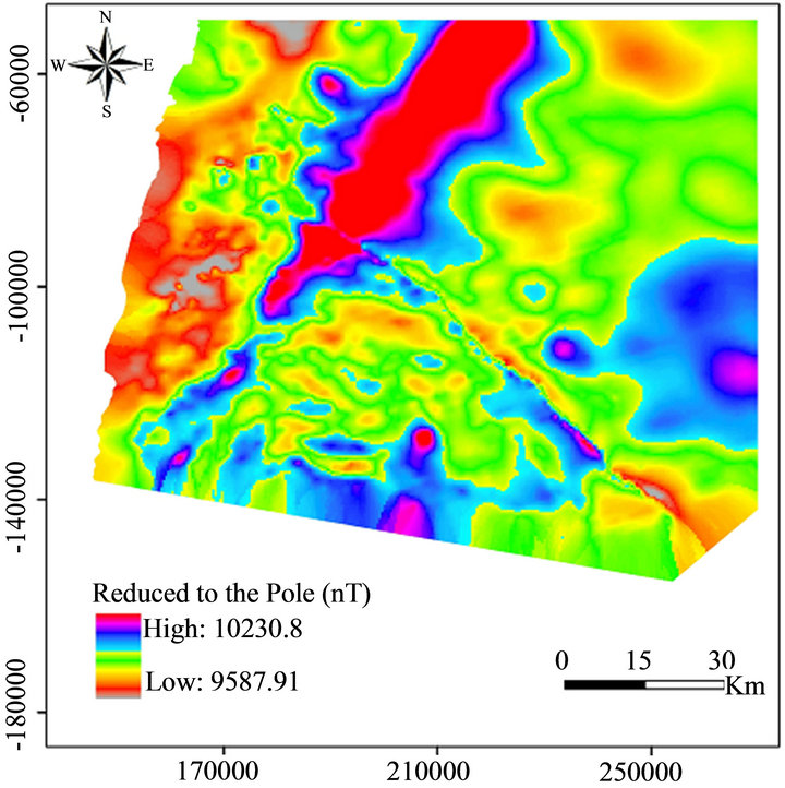
Figure 6. Reduced to the magnetic pole map.
depths. It shows several dominant trends generally, aligned along definite axis that can be used to define the magnetic provinces. The most dominant trend is the NW-SE and the, NE-SW directions. In addition, several minor small high and low magnetic features were found to trend in E-W direction.
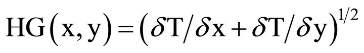
3.1.3. Horizontal Gradient
The enhancement of magnetic anomalies associated with the faults and other structural discontinuities was achieved by the application of band pass filter, and calculating the horizontal derivative of the aeromagnetic datasets. The horizontal gradient (HG) can be defined as follows, if T(x,y) is the magnetic field and the horizontal derivatives of the field in x and y directions are (δT/δx, and δT/δy) respectively, then the Horizontal Gradient HG (x,y) is given by [11]:
 (1)
(1)
The horizontal gradient (HG) method is considered as the simplest method approach to estimate the contact locations (e.g. faults) [11]. The horizontal gradient map aided in defining the locations of the faults which in turn were related to fault trend and fractures in the area. The HG method was applied to the aeromagnetic dataset at different azimuths using Geosoft Package (V.6.4.2). The results were incorporated into GIS environment and presented in Figures 7 and 8. It displays detailed information about the structures, contacts and the tectonic setting of the study area.
3.1.4. Vertical Gradient
The vertical derivative (gradient) operator is often applied
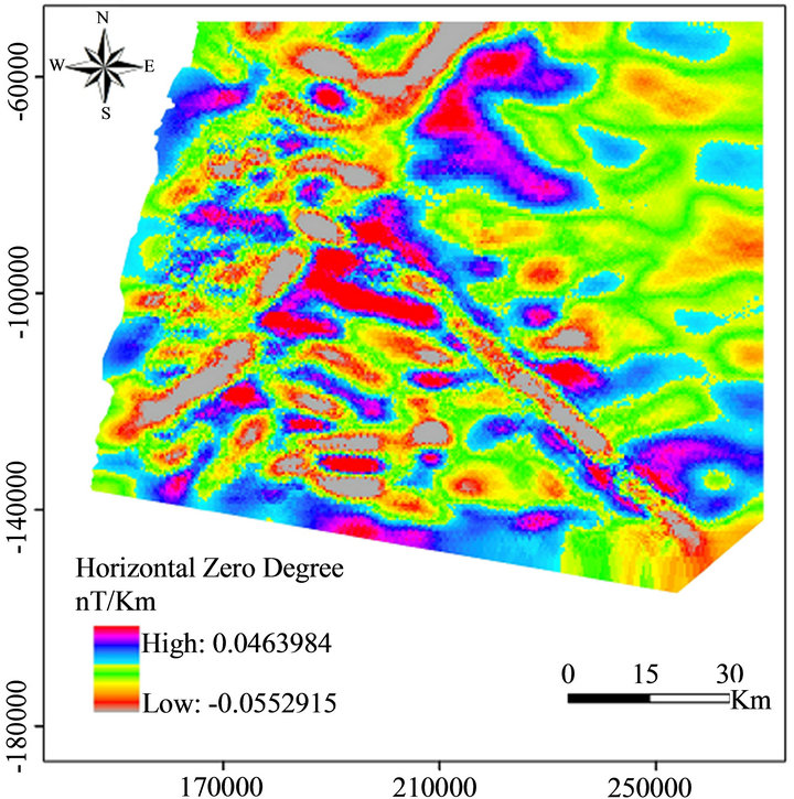
Figure 7. Horizontal zero degree magnetic field map.
Figure 8. Horizontal 90˚ magnetic field map.
to ground or airborne magnetic data to sharpen the edges of anomalies and other significant features [10]. The algorithm is given by Gunn [12]:
 (2)
(2)
where A (u,v) is the amplitude present at those frequentcies, and n is the order of the derivative. The higher the order of derivative, the noisier the map will become [10]. The first vertical gradient of aeromagnetic data was calculated using Geosoft package V.6.4.2, incorporated into the GIS Environment, and presented in Figure 9.
3.1.5. Analytical Signal
The analytical signal of the magnetic anomaly field can be effectively used to map the edges of 3-D and 2-D bodies [13]. This method is based on the use of the spatial derivatives of magnetic anomalies (F(x,y)) computed along three orthogonal directions [14]. By this operation the total absolute value of analytical signal  of a given magnetic anomaly field can be obtained by summing the three square differentials [15]:
 (3)
(3)
The analytical signal displays the maxima over 2-D source body edges even when the direction of magnetization is not vertical [15]. In this study, the analytical signal of the aeromagnetic data was calculated using Geosoft package V.6.4.2 and the result is incorporated into GIS environment and presented in Figure 10. The
Figure 9. Vertical gradient magnetic field map.
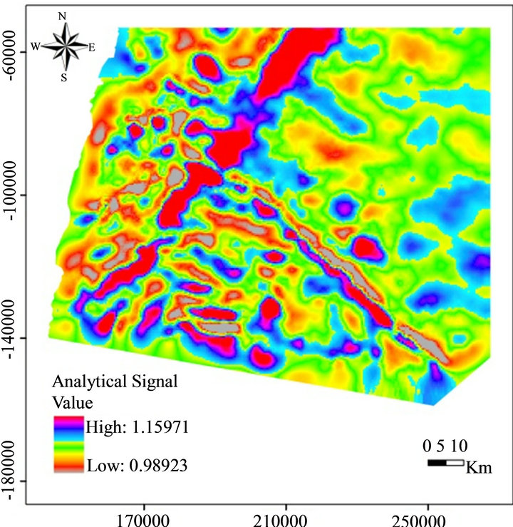
Figure 10. Analytical signal magnetic field map.
structural features, aeromagnetic lineaments, and their different alignments in the study area were deduced from the different geophysical maps Figure 11.
3.1.6. Euler Deconvolution
Euler deconvolution [16] is a method to estimate the depth of subsurface magnetic anomalies and can be applied to any homogeneous field, such as the analytical signal of magnetic data [17]. It is particularly good at delineating the subsurface contacts. It has been observed that the depth estimates from magnetic data are more
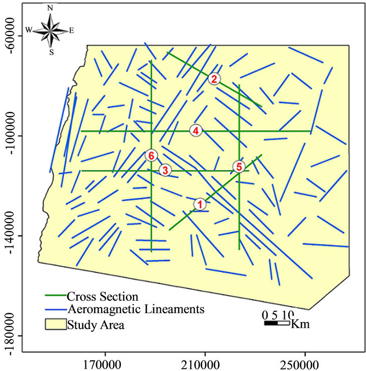
Figure 11. Aeromagnetic lineaments map and location of cross section profiles.
accurate if the pole-reduced magnetic field is used [18], than using the magnetic data themselves.
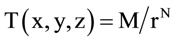
In this study, the reduced to the magnetic pole map was used to map the subsurface structures and contacts using EULDEP software [17]. This software is based on calculating the horizontal and vertical gradients of the magnetic field (RTP in this case) along profile data [17]. The method is an automatic depth estimates one, and is designed to provide computer assisted-analysis on large volumes of magnetic data [19]. In addition, to making use of the property of the rapid decay of intensity of magnetization with distance from the source. The intensity of magnetization or magnetic field 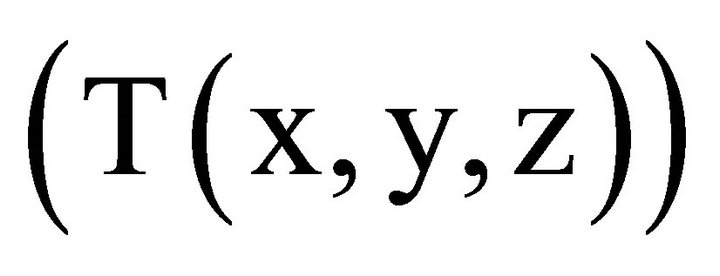 as a result of the distribution of magnetic poles can be written as follow:
 (4)
(4)
where r is , M is proportional to magnetization and N is the structural index with values ranging from 0 to 3 [17].
In this Study, different aeromagnetic profiles with different orientations Figure 11 distributed over the study area and crossing the major magnetic anomalies have been constructed processed with different structural indices Table 1 and interpreted in terms of sub-surface structures Figure 12.
The dataset for each profile has been digitized with the aid of GIS techniques. The profile data were then processed using the EULEDEP software. In addition, the surface fault traces from surface detailed geological maps were mapped and delineated using GIS techniques along each profile and were incorporated along with the results
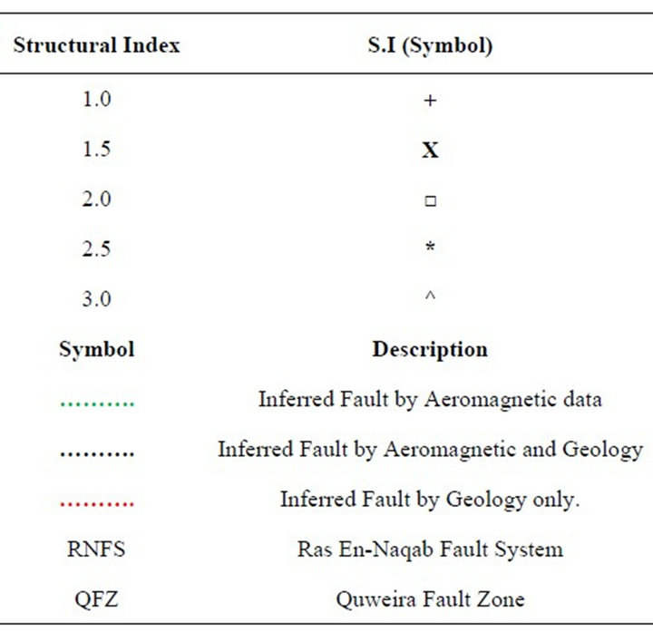
of the processed profile data (Figure 12, Red and Green dashed lines). The results show that, several subsurface faults have been inferred from the modeled aeromagnetic profiles data which were not documented in surface geological maps (Black dashed lines, Figure 12). Some of the delineated geological faults were not detected by modeled aeromagnetic profile data (Red dashed lines, Figure 12). But, most of the delineated geological faults were found coincident with the interpreted aeromagnetic faults (Green dashed lines, Figure 12(e) and Figure 12). Moreover, the modeled aeromagnetic profiles data showed that the inferred faults may extend downward for several kilometers.
3D Euler solution for the aeromagnetic data of the study area, at Structural Index (S.I = 1) have been produced using the GEOSOFT packages and the result is presented in Figure 13.
3.2. Landsat Interpretation
Four scenes of Landsat ETM+ images were downloaded from USGS website that covers the study area. These images were converted into PIX format to become suitable for PCI Geomatics 9.1 software. Mosaic and subset operations were performed to clip the images for the study area Figure 14.
Available structural maps were also used in this study. However, automated lineament extraction techniques had to be used to increase the details of existing data of structural maps. The main advantages of automated lineament extraction over the manual lineament extraction are; the ability to uniformly approach the different images; processing operations are performed in a short
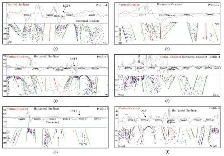
Figure 12. Sub-surface structural interpretation and magnetic causative anomalies.
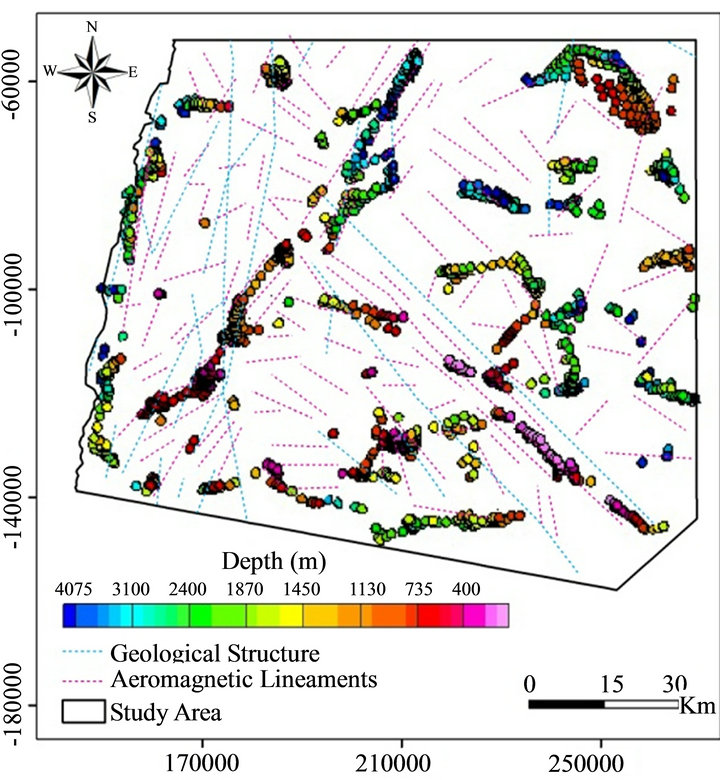
Figure 13. 3D Euler solution from the analysis the aeromagnetic data over the study area, with structural index (S.I = 1) combined with geological and inferred aeromagnetic structures.
Figure 14. Land sat ETM+ imagery for the study area.
time, and the ability to extract lineaments which are not recognized by human eyes. This was done by applying LINE module of PCI Geomatica 9.1 software. This module extracts linear features from an image and records the polylines in vector segments by using six parameters. These parameters are (PCI Geomatics 9.1 Users Manual):
1) RADI (Filter radius): This parameter is used in the first step of the first stage of the process for the “Canny edge detection”. It specifies the radius of the edge detection filter (in pixels), and roughly determines the smallest-detail level in the input image to be detected.
2) GTHR (Gradient threshold): This parameter is used in the second stage of the process for the “Canny edge detection”. It specifies the threshold for the minimum gradient level for an edge pixel to obtain a binary image.
3) LTHR (Length threshold): This parameter is used in the third stage of the process. It specifies the minimum length of curve (in pixels) to be considered as lineament or for further consideration (e.g., linking with other curves).
4) FTHR (Line fitting error threshold): This parameter is used in the second step of the third stage. It specifies the maximum error (in pixels) allowed in fitting a polyline to a pixel curve. Low FTHR values give better fitting but also shorter segments in polyline.
5) ATHR (Angular difference threshold): This parameter is used in the last step of the third stage of the process. It specifies the maximum angle (in degrees) between segments of a polyline. Otherwise, it is segmented into two or more vectors. It is also the maximum angle between two vectors for them to be linked.
6) DTHR (Linking distance threshold): This parameter is used in the last step of the third stage of the process. It specifies the minimum distance (in pixels) between the end points of two vectors for them to be linked. The used parameters and their values appear in Table 2.
Figure 15 shows the results obtained by applying the LINE module.
3.3. Discussion and Conclusions
The extracted Landsat lineaments Figure 15 and inferred aeromagnetic lineaments Figure 11 have been investigated and correlated using frequency rose diagram in a GIS environment for different parts of the study area and for the whole study area Figure 16. Two main lineament sets were observed in the study area, with the major orientations of the lineament sets in NW-SE and NE-SW directions and a minor set in E-W direction Figure 16. General coincidence of both Landsat and aeromagnetic lineaments trends is observed in the study area Figure 16
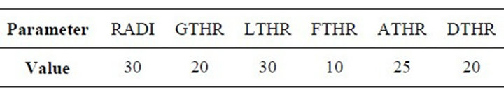
Table 2. Parameters used in LINE module.
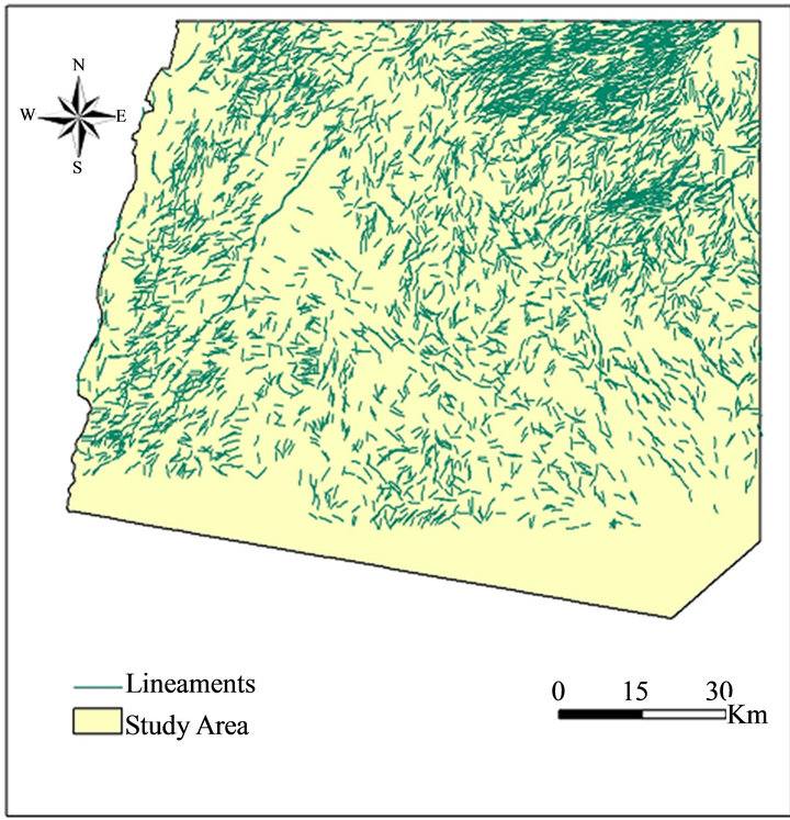
Figure 15. Extracted lineaments using LINE module.
which means that, these lineaments reflect real continuous fractures in depth. The NW-SE and NE-SW lineament sets are the most frequent and are more conspicuous in the study area. The NW-SE set of fractures is present in most parts of the study area. This set represents the extensional fractures as they parallel faults like Ras En-Naqab and Mudawwara which cross the study area in a NW-SE direction with more than 100 km length Figure 3. The set is assumed to be a pre-rift structure belonging to the opening of the Red Sea, and is sub-parallel to the Red Sea system.
The NE-SW to NNE-SSW lineaments trend set dominate the study area. This trend represents the compressional and P-shear fractures related to the movement of the DST and the Dead Sea stress field in the region ([20,21]).
The general E-W lineaments trend set of local distribution represents the conjugate Riedel shear fractures like dextral strike-slip faults. Strike-slip faults dominate the study area in its western parts Figures 3, 11 and 16. These faults are oriented N-S and are represented mainly by the Al-Quweira sinistral strike-slip fault zone and other sub-parallel smaller faults which in turn non sub-parallel to the Dead Sea transform Figure 3 and Figure 16. The N-S trending lineaments have local distribution and are the youngest trend in the study area as they cut the other trends. They are covered by Pleistocene to Holocene sediments, which explain the weak trend of lineaments in this direction Figure 16 in spite of the dominating faults shown in the structural map Figure 3. Each trend of these faults is accompanied by parallel and sub-parallel sets of joints of smaller scale and can
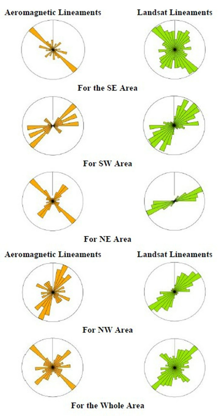
Figure 16. Frequency rose diagrams for the deduced lineaments for both the aeromagnetic lineaments and lineaments deduced from Landsat Imagery in the different parts of the study area as well as for the whole study area.
not be observed in satellite images. The 3D Euler solution of the study area shows that the depth of magnetic source body ranges from hundreds of meters (light to dark Pink in Figure 13) in the central and southeastern part of the study area to more than 3000 m in the middle northern part of the study area (Blue circles, Figure 13). The 3D Euler solution reflects the topography of the basement and its associated structures. The increase in the depth of the source magnetic body towards the northern and northeastern parts of the study area is correlated with the emplacement of basement rocks in south Jordan and its NE dipping nature [5].
REFERENCES
- A. S. Al-Zoubi and Z. Ben Avraham, “Structure of the Earth’s Crust in Jordan from Potential Field Data,” Tectonophysics, Vol. 346, No. 1-2, 2002, pp. 45-59. doi:10.1016/S0040-1951(01)00227-X
- R. D. Hatcher, I. Zeitz, R. D. Regan and M. Abu-Ajamieh, “Sinistral Strike-Slip Motion on the Dead Sea Rift: Confirmation from New Magnetic Data,” Geology, Vol. 9, No. 10, 1981, pp. 458-462. doi:10.1130/0091-7613(1981)9<458:SSMOTD>2.0.CO;2
- M. Barjous and S. Mikbel, “Tectonic Evolution of the Gulf of Aqaba-Dead Sea Transforms Fault System,” Tectonophysics, Vol. 180, No. 1, 1990, pp. 49-59. doi:10.1016/0040-1951(90)90371-E
- A. Diabat and A. Masri, “Orientation of the Principal Stresses along Zerqa-Ma’in Fault,” Mu’tah Lil-Buhuth wad-Dirasat, Vol. 20, No. 1, 2005, pp. 57-71.
- F. Bender, “Geology of Jordan,” Borntraeger Press, Berlin, 1974.
- Phoenix Corporation, “A Comprehensive Airborne Magnetic/Radiometric Survey of the Hashemite Kingdom of Jordan,” Final Report to Natural Resources Authority, Jordan, 1981.
- M. Hassouneh, “Jordan Aeromagnetic Map, Scale 1:500,000,” Natural Resources Authority, Jordan, 1998.
- R. O. Hansen and R. S. Pawlowski, “Reduction to the Pole at Low Latitudes by Weiner Filtering,” Geophysics, Vol. 54, No. 12, 1998, pp. 1607-1613. doi:10.1190/1.1442628
- V. Chandler, J. Koski, W. Hinze and L. Braile, “Analysis of Multi Sources Gravity and Magnetic Anomaly Data Sets by Moving-Windows Application of Poisson’s Theorem,” Geophysics, Vol. 46, No. 1, 1981, pp. 30-39. doi:10.1190/1.1441136
- R. J. Cooper, “GravMap and PFproc: Software for Filtering Geophysical Map Data,” Computer and Geosciences, Vol. 23, No. 1, 1997, pp. 91-101. doi:10.1016/S0098-3004(96)00064-7
- J. D. Phillips, “Processing and Interpretation of Aeromagnetic Data for the Santa Cruze Basin-Patagonia Mountain Area, South Central Arizona,” US Geological Survey Open-File Report 02-98, 2001.
- P. J. Gunn, “Linear Transformation of Gravity and Magnetic Fields,” Geophysical Prospecting, Vol. 23, No. 2, 1975, pp. 300-312. doi:10.1111/j.1365-2478.1975.tb01530.x
- W. R. Roest, J. Verhoef and M. Pilkington, “Magnetic Interpretation Using 3-D Analytical Signal,” Geophysics, Vol. 57, No. 1, 1992, pp. 116-125. doi:10.1190/1.1443174
- R. Lanza and A. Meloni, “The Earth’s Magnetism—An Introduction for Geologists,” Springer-Verlag, Berlin, Heidelberg, 2006.
- P. V. Sharma, “Environmental and Engineering Geophysics,” New York, 1997. doi:10.1017/CBO9781139171168
- A. B. Ried, J. M. Allsop, H. Granser, A. J. Millett and I. W. Somerton, “Magnetic Interpretation in Three Dimensions Using Euler Deconvolution,” Geophysics, Vol. 55, No. 1, 1990, pp. 80-91. doi:10.1190/1.1442774
- R. J. Durrheim and R. J. Cooper, “EULDEP: A Program for the Euler Deconvolution of Magnetic and Gravity Data,” Computer and Geosciences, Vol. 24, No. 6, 1998, pp. 545-550. doi:10.1016/S0098-3004(98)00022-3
- D. T. Thomson, “Euldph: A New Technique for Making Computer Assisted Depth Estimates from Magnetic Data,” Geophysics, Vol. 47, No. 11, 1982, pp. 31-37. doi:10.1190/1.1441278
- M. G. El-Dawi, L, Tianyou, H. Shi and L. Dapeng, “Depth Estimation of 2-D Magnetic Anomalous Sources by Using Euler Deconvolution Method,” American Journal of Applied Sciences, Vol. 1, No. 3, 2004, pp. 209-214. doi:10.3844/ajassp.2004.209.214
- A. Diabat, “Paleostress and Strain Analysis of the Cretaceous Rocks in the Eastern Margin of the Dead Sea Transform, Jordan,” Ph.D. Dissertation, University of Baghdad, Baghdad, 1999.
- A. Diabat, M. Atallah and M. Salih, “Paleostress Analyses of the Cretaceous Rocks in the Eastern Margin of the Dead Sea Transform,” Journal of African Earth Sciences, Vol. 38, No. 5, 2004, pp. 449-460. doi:10.1016/j.jafrearsci.2004.04.002
NOTES
*Corresponding author.