Natural Science
Vol.6 No.5(2014), Article ID:43472,16 pages DOI:10.4236/ns.2014.65030
Mathematical Model of Cell Growth for Biofuel Production under Synthetic Feedback
Ondivillu Mothilal Kirthiga, Lakshmanan Rajendran
Department of Mathematics, The Madura College, Madurai, India
Email: raj_sms@rediffmail.com
Copyright © 2014 by authors and Scientific Research Publishing Inc.
This work is licensed under the Creative Commons Attribution International License (CC BY).
http://creativecommons.org/licenses/by/4.0/


Received 10 January 2014; revised 10 February 2014; accepted 17 February 2014
ABSTRACT
In this paper, mathematical model for cell growth and biofuel production under synthetic feedback loop is discussed. The nonlinear differential equations are solved analytically for the maximum production of biofuel under synthetic feedback. The closed-form of analytical expressions pertaining to the concentrations of cell density, repressor proteins, pump expressions, intracellular biofuel and extracellular biofuel are presented. The constant pump model is compared with feedback loop model analytically to know the biofuel production. The numerical solution of this problem is also reported using Scilab/Matlab program. Also, the analytical results are compared with previous published numerical results and found to be in good agreement.
Keywords:Mathematical Modeling; Non-Linear Equations; Biofuel; Feedback Loop; Biosensor

1. Introduction
Micro-organisms (or microbes) play a very important role in our lives. Some microbes cause disease but the majority is completely harmless. Microbes help as for the production of enzymes and chemicals. In particular, most common biofuel is ethanol, which is produced from the plants. Breakdown of cellulous will also form ethanol. However, there are numerous scientific and technical challenges involved with utilizing lignocelluloses material for biofuel production.
Biological and biochemical processes have a very important role in medicine, biology and biotechnology. However, it is very difficult to convert directly biological data to electrical signal; the biosensors can convert these signals and the biosensors over this difficulty [1] . The advantages of biosensors such as cost-effectiveness, specificity of detection, portability reduced overall time required for detection. Clark et al. [2] developed the first biosensor, an enzyme based glucose sensor. Then so many biosensors are developed in many research laboratories [3] .
The cell growth and biofuel production implement a synthetic feedback loop using a biosensor to control efflux pump expression. In this way, the production rate will be maximal when the concentration of biofuel is low because the cell does not expend energy expressing efflux pumps when they are not needed. Efflux pumps identify harmful compounds; transfer them from the cell using the proton motive force and have proven effective at exporting biofuel. Even though they improve tolerance, if over expressed, efflux pumps can be harmful. By using efflux pumps giving to increase tolerance to biofuel, pump toxicity managed biofuel toxicity. Feedback is a common mechanism to adjust the conditions such as environmental stressors and signals from other cells. Synthetic feedback helps to control efflux pump expression which would balance the toxicity of biofuel production against the adverse effect of pump expression.
Clomburg et al. [4] discussed that synthetic biology will help improve the productivities of biofuels. The mechanism of microbes causes unwanted cellulose stress that leads to over production of proteins which results in decreases of cell fitness. Fisher et al. [5] tested seven fast growing host organisms for biofuel production which tolerate production stresses. Mostafa et al. [6] provided a brief overview on the research in the area of biofuels, with specific emphasis on the economic viability of various approaches.
Peralta et al. [7] concentrated on the metabolic engineering of genetically polite organisms such as Escherichia coli and Saccharomyces cerevisiae for the production of these advanced biofuels. Soto et al. [8] studied the importance of efflux pumps in biofilm growth and about their relevance in antimicrobial resistance forming biofilm. Huffer et al. [9] highlighted recent advances in metabolic engineering of biofuel-synthesis pathways in E. coli and summarized insights gained into regulation of those pathways, and described progress toward overcoming the challenges facing its adoption as a biofuel-production strain. Christopher et al. [10] discussed the contributions of systems biology for the purpose of utilizing microorganisms for biofuel production.
Recently, Dunlop et al. [11] developed a model for cell growth and biofuel production. Harrison et al. [12] developed a mathematical model for cell growth and biofuel production that implement a synthetic feedback loop using a biosensor to control efflux pump expression. To the best of our knowledge, there is no general analytical expression for the concentration of cell density, repressor proteins, pump expressions, intracellular biofuel and extracellular biofuel against the time t. The purpose of this paper is to derive an analytical expression for the concentrations of cell density, repressor proteins, pumps, intracellular biofuel and extracellular biofuel for both steady and non-steady state conditions.
2. Mathematical Formulation of the Problem
2.1. Feedback Loop Model
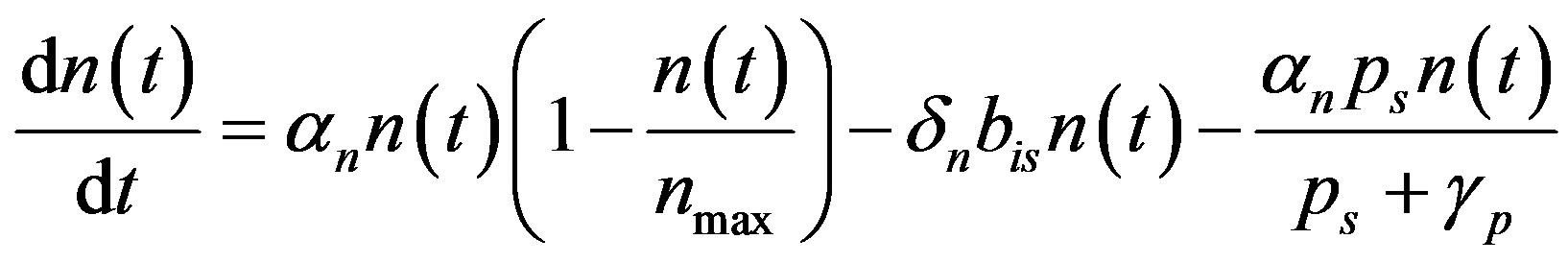
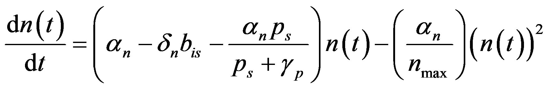
The complete mathematical formulation of this problem is described in [12] . This model involves five nonlinear differential equations with limited number of parameter are described as follows [12] :
 (1)
(1)
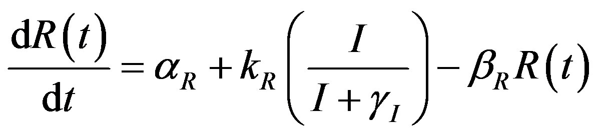 (2)
(2)
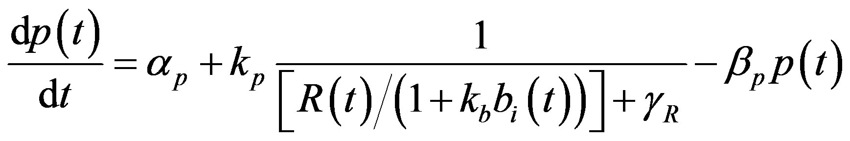 (3)
(3)
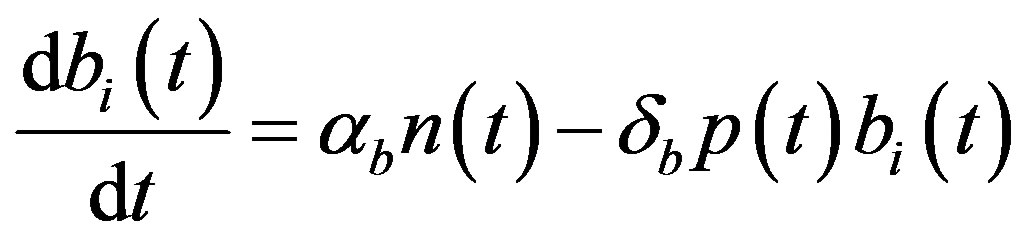 (4)
(4)
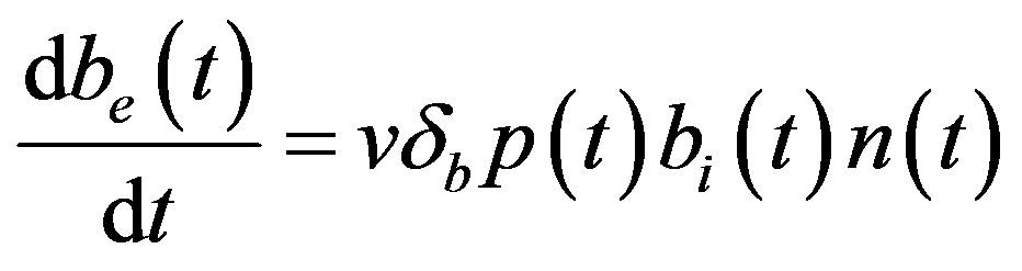 (5)
(5)
Here  and
and  denote concentrations of cell density, repressor proteins, pumps, intracellular biofuel and extracellular biofuel respectively. Delay in cell growth is happens due to biofuel toxicity
  and pump toxicity
 . When the promoter is not activated,
  and
and  represents the low level of expression.
  and
and  represent the degradation rates.
  and
and  represent the strength of expression for R and
 , respectively. In Equation (3),
  represents the repression of efflux pump expression and
  represents the amount of active
  in the system. The parameter
  represents the deactivation constant of
 . Repressor activation by the inducer IPTG is modeled as
 , where
  indicates the inducer value that corresponds to half maximal activation of repressor. Amount of inducer is proposional to the repressor concentration. The initial conditions are given by.
At
 (6)
(6)
The steady state expressions of the concentrations for this model are obtained as follows:
 (7)
(7)
 (8)
(8)
 (9)
(9)
 (10)
(10)
where ,
,

and other parameters are in Table 1.
Analytical Expressions of the Concentrations of Cell Density, Repressor Proteins, Pumps, Intracellular and Extracellular Biofuel
By solving the non-linear Equations (1)-(5) using Homotopy perturbation method (Appendix A) [13] -[18] , the analytical expressions of the concentrations of cell density, repressor proteins, pumps, intracellular and extracellular biofuel are obtained for non-steady state as follows:
 (11)
(11)
 (12)
(12)
 (13)
(13)
 (14)
(14)
 (15)
(15)
where
 (16)
(16)

Table 1. Symbols used.
Continued
The Equations (11)-(15) represent new analytical expressions for the concentrations of cell density, pumps, intracellular and extracellular biofuel for this model.
2.2. Constant Pump Model
For this model, the concentration of repressor proteins  is removed and the concentration of cell density
 , intracellular biofuel
  and extracellular biofuel
  remains the same. But the concentration of pumps expression
  becomes
 (17)
(17)
where the value of I (IPTG) is selected from 0 mM to 1 mM. We can obtain the steady state expressions of concentrations for constant pump model as follows:
 (18)
(18)
 (19)
(19)
 (20)
(20)
Analytical Expressions of the Concentrations of Cell Density, Pumps, Intracellular and Extracellular Biofuel
By solving the Equations (1), (4), (5) and (17), the closed form of an analytical expression of the concentrations of pumps, intracellular biofuel and extracellular biofuel are obtained as follows:
 (21)
(21)
 (22)
(22)
 (23)
(23)
 (24)
(24)
where
 (25)
(25)
The Equations (21)-(24) represents new analytical expressions for the concentrations of cell density, pumps, intracellular and extracellular biofuel for constant pump model.
3. Numerical Simulation
The non-linear differential Equations (1)-(5) are solved by numerical method. The function pdex4 in Scilab software which is a function of solving partial differential equations (PDE) is used to solve these equations. To show the efficiency of the present method, our analytic results are compared with numerical solution and it gives a satisfactory agreement. The SCILAB/MATLAB program is also given in Appendix B.
4. Discussion
Equations (11)-(15) represents simple analytical expressions for the concentrations of cell density, pumps, intracellular and extracellular biofuel in terms of six parameters, biofuel export rate , biofuel toxicity coefficient
 , biofuel production rate
 , growth rate
 , pump toxicity threshold
 , and maximum cell density
 . Those parameters give the greatest impact on the system when they are varied. Production of biofuel depends upon the growth rate, maximum cell density, pump toxicity threshold and biofuel toxicity coefficient.
Simulation results are often used to validate the analytical solutions. Recently, Harrison et al. [12] obtained the numerical solution of the nonlinear equations in feedback model using MATLAB program. The Figure 1 shows cell density , pump
 , intracellular biofuel
 , extracellular biofuel
  versus time
 . In this figure, our analytical results are compared with the simulation results. Our analytical results were found to be in satisfactory agreement with simulation results.
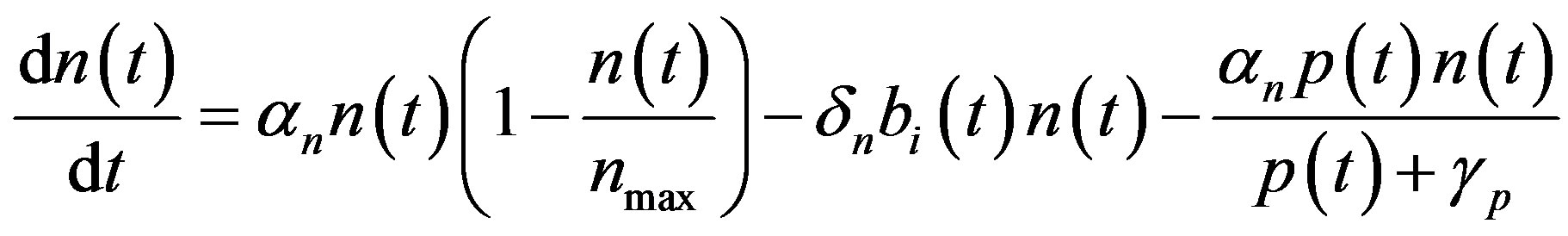
Figure 2 represents the cell density  versus time t. The concentration depends upon the pump toxicity threshold
 , biofuel toxicity coefficient
 , maximum population size
  and growth rate
 . After very short time, cell density increases sharply and reaches the maximum value nearly 0.4 after 25 hours. Also from this figure, it is including that the cell density increases when growth rate is decreases and coefficient of biofuel toxicity is increases.
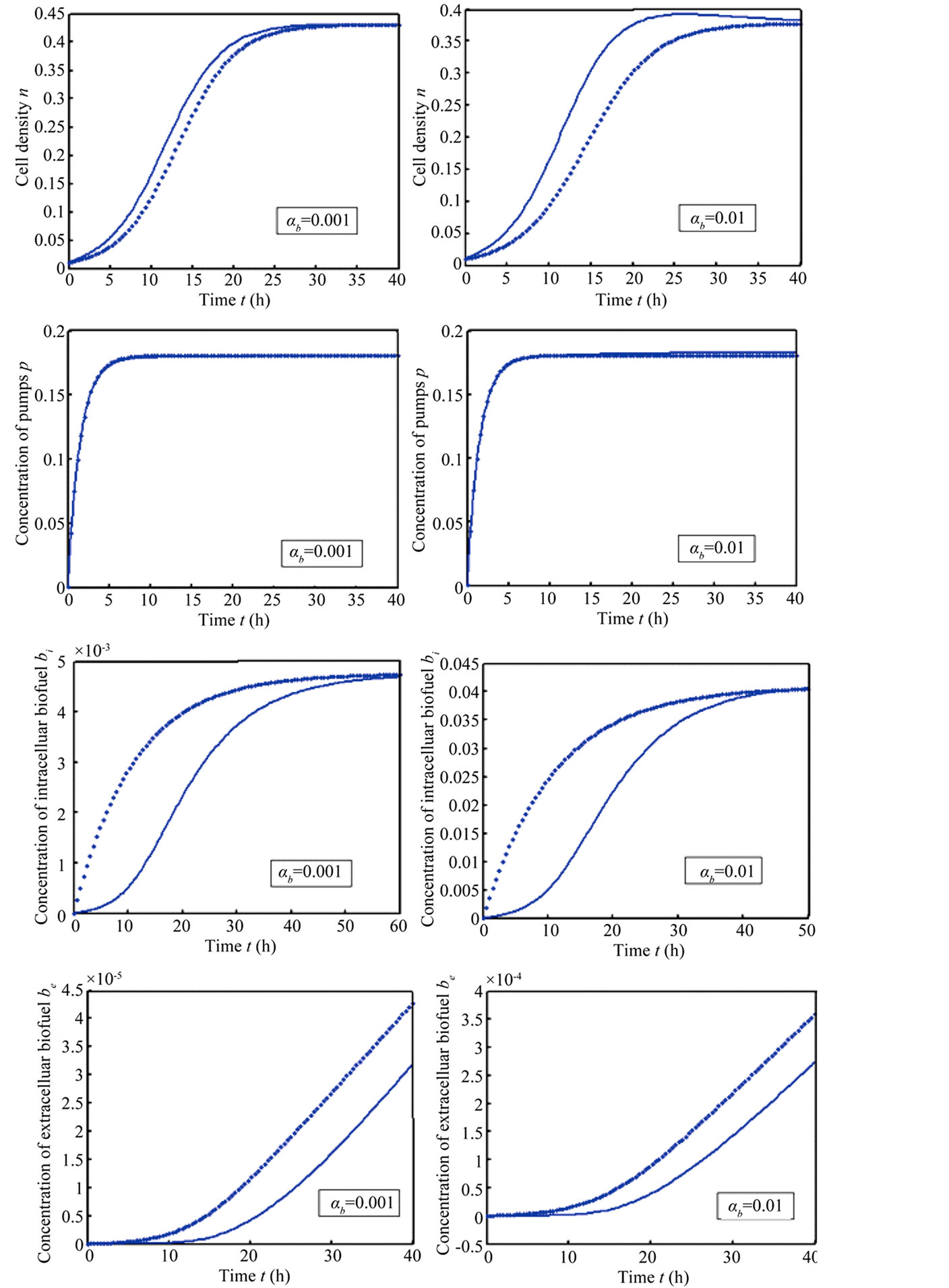
Figure 1. Comparison of analytical results (feedback model) with previous numerical results (Harrison et al., [12] ): The concentrations were computed using Equations (11)-(15) for the experimental values. The key to the graph: dotted line represents the analytical results and solid line represents the numerical results.
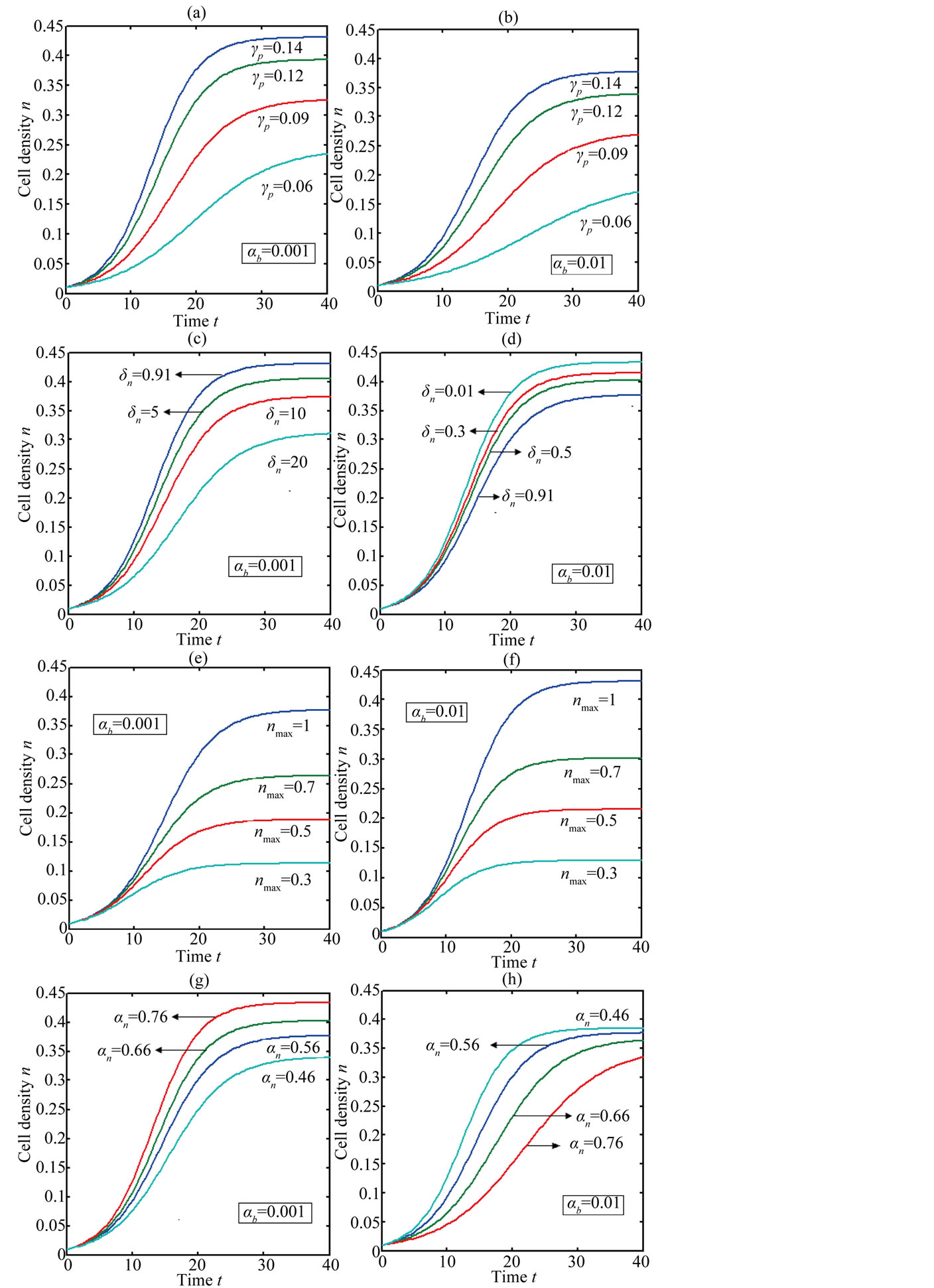
Figure 2. Cell density n(t) versus time t for various values of pump toxicity threshold γp, biofuel toxicity coefficient δn, maximum population size nmax and growth rate αn and for some fixed values of the parameters (refer Table 1).
The concentration of repressor  with time t for various values of repressor degradation rate
 , repressor activation constant
  and basal repressor production rate
  is shown in Figure 3. When time increases the concentration also increases and finally it reaches the steady state value at short time
 . Repressor prevents efflux pump expression until it is deactivated by biofuel.
In Figure 4, the concentration of pumps  measured with time t for various experimental values of repressor saturation threshold
 , pump activation constant
 , pump degradation rate
  and basal pump production rate
 . If time increases the concentration also increases and finally it reach steady state level by the control of efflux pump using feedback model. Pump expression increases the biofuel productions because of repressor deactivation. Concentration of pump depends upon the rate of pump expression.
Figure 5 describes the intracellular biofuel  with time t. For both biofuel production rate, when time t increases concentration of intracellular biofuel also increases. Biofuel rate is increased because intracellular biofuel accumulates more quickly and efflux pumps are needed earlier.
Figure 6 indicates the extracellular biofuel  versus time t. The concentration depends upon biofuel export rate per pump
 , ratio of intra to extracellular volume
  and cell growth rate
 . For both biofuel production rate, if time increases the concentration also increases. From this figure, it is observed that the concentration of extracellular biofuel linearly increases with time t. This is because when efflux pumps are used to export biofuel form the cell the extracellular level of biofuel will increase, allowing intracellular biofuel levels to remain low.
An analytical expression of cell density , concentration of pump
 , intracellular biofuel
  and extracellular biofuel
  for feedback and constant pump model are compared in Figure 7. This figure
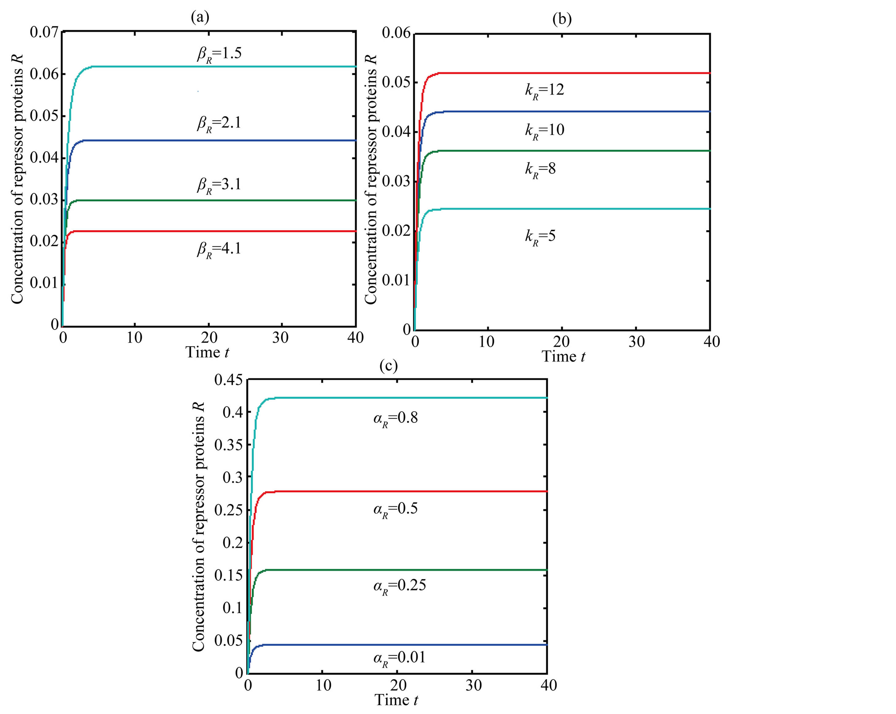
Figure 3. Concentration of repressor proteins R(t) versus time t for various values of repressor degradation rate βp, repressor activation constant kR and basal repressor production rate αR and for some fixed values of the parameters (refer Table 1).
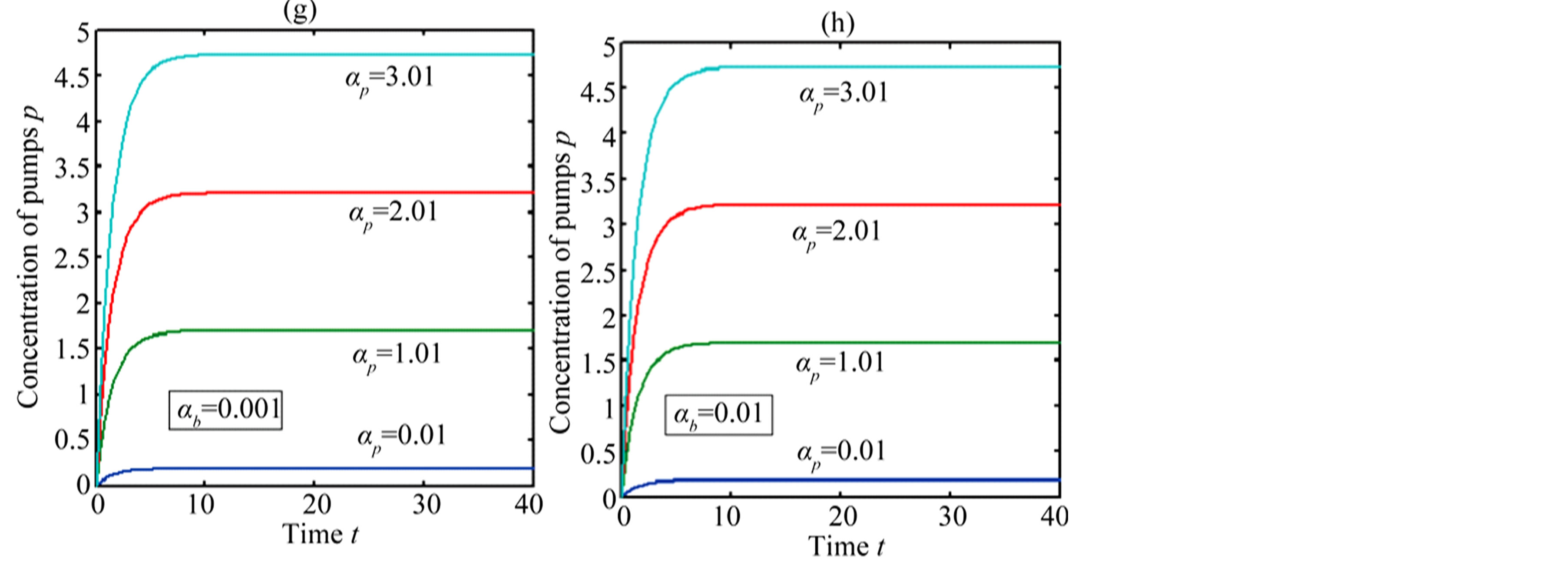
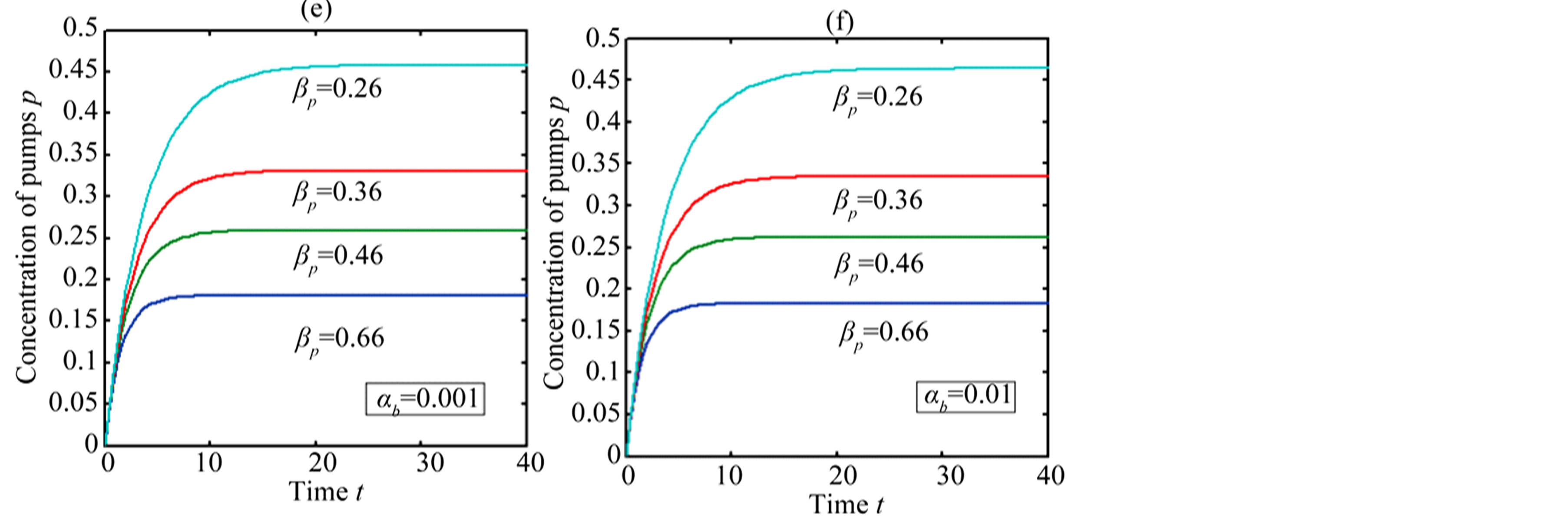
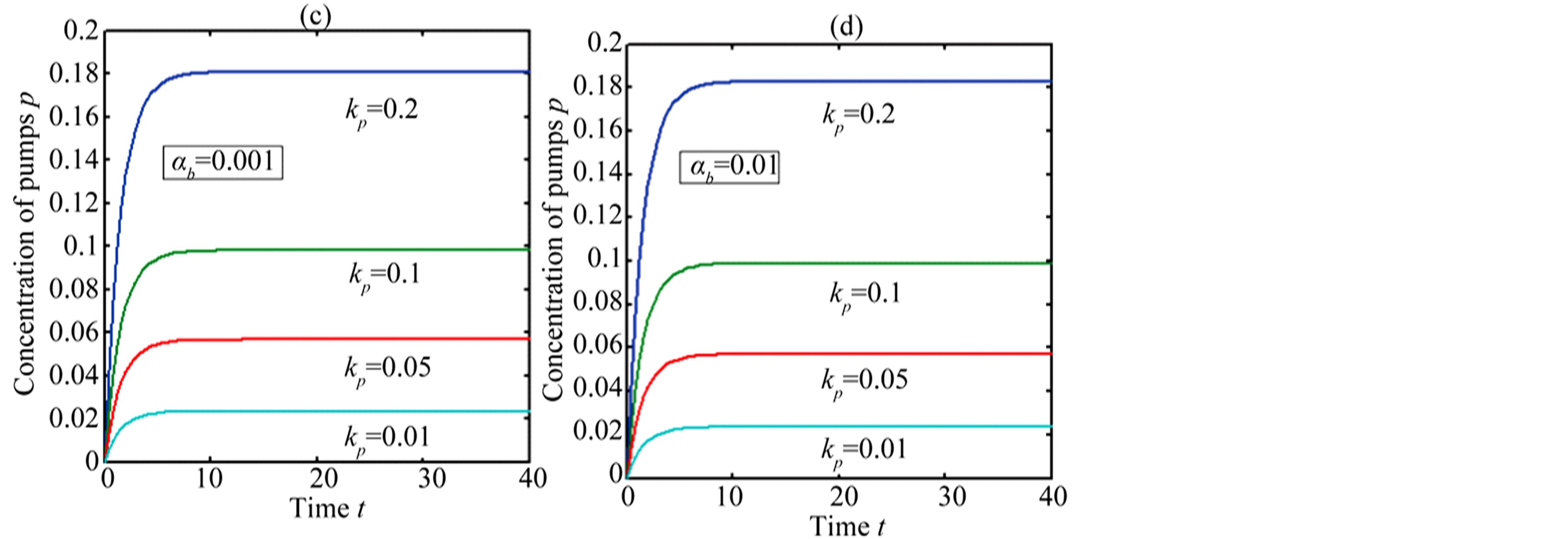
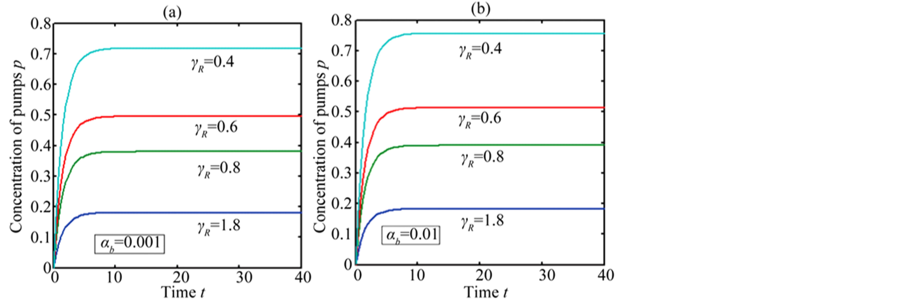
Figure 4. Concentration of pumps p(t) versus time t for various values of repressor saturation threshold γR, pump activation constant kp, pump degradation rate βp and basal pump production rate αp and for some fixed values of the parameters (refer Table 1).
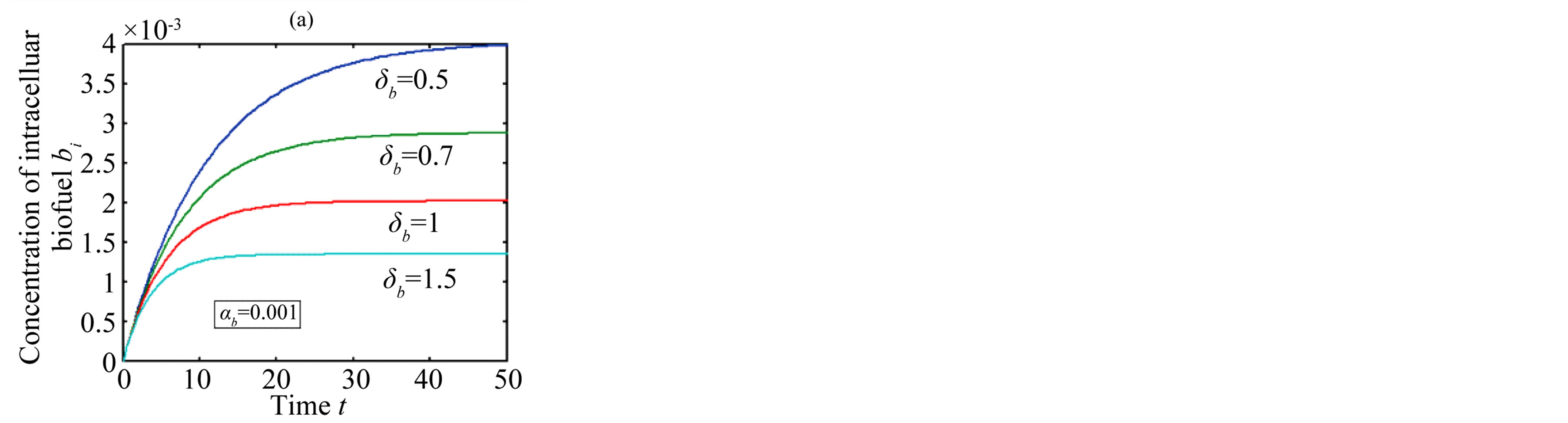
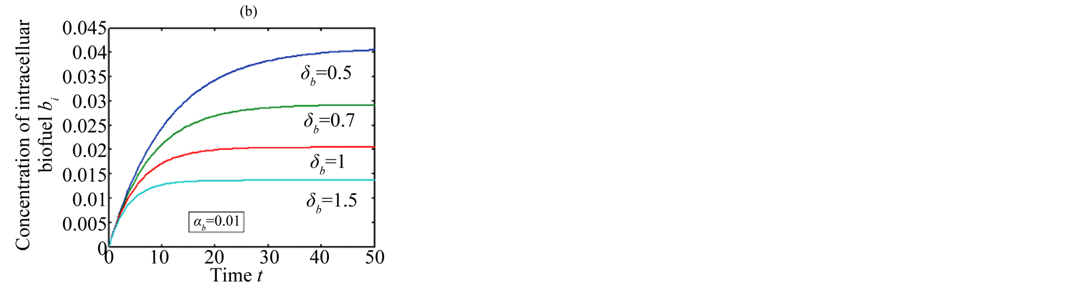
Figure 5. Concentration of intracellular biofuel bi(t) versus time t (a) At αb = 0.001 for various values of biofuel export rate per pump δb and some fixed experimental values of other parameters. (b) At αb = 0.01 for various values of δb and some fixed experimental values of other parameters.

Figure 6. Concentration of extracellular biofuel be(t) versus time t for various values of biofuel export rate per pump δb, ratio of intra to extracellular volume  and cell growth rate αn and for some fixed values of the parameters (refer Table 1).
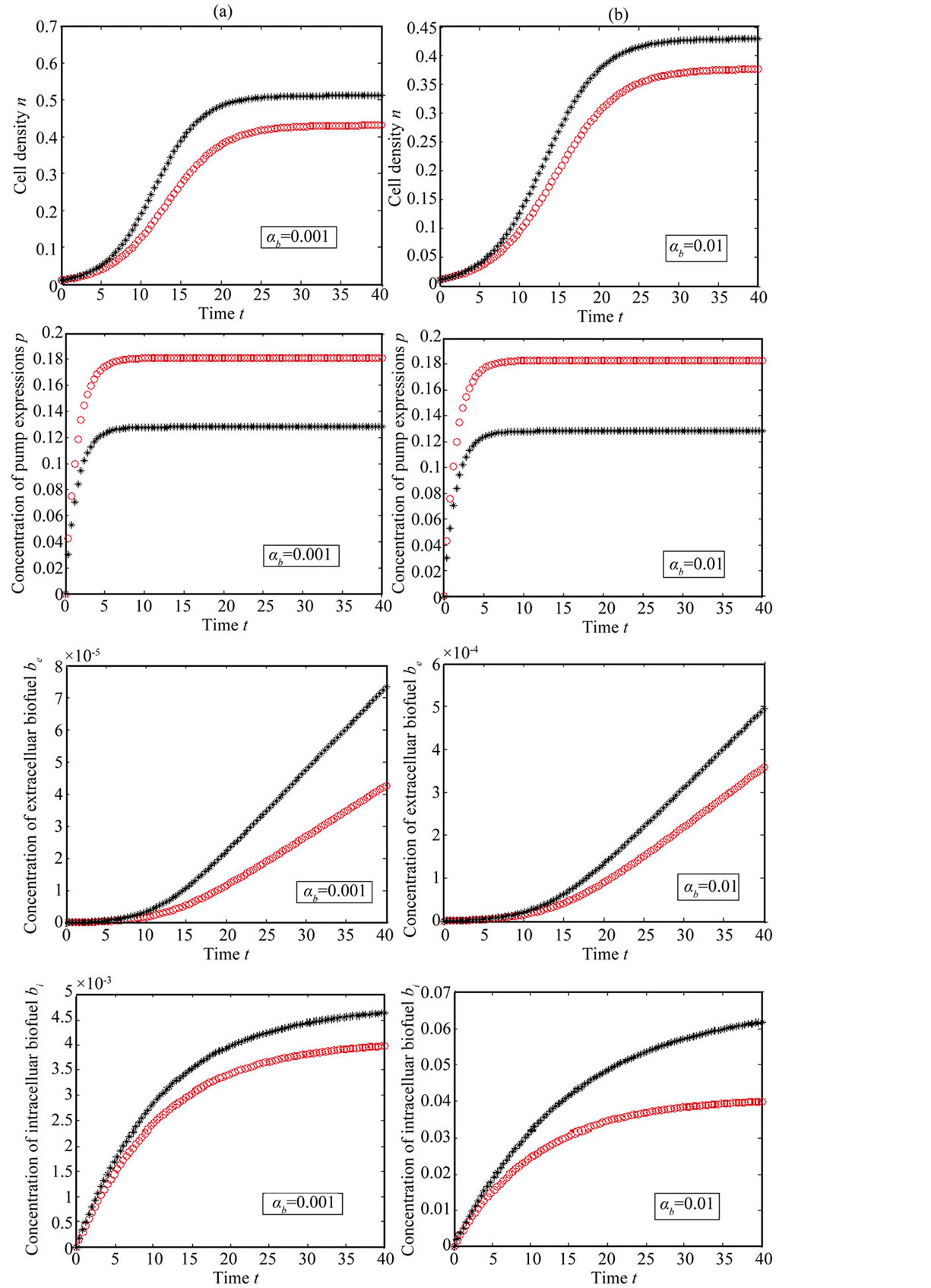
Figure 7. Comparision of concentrations for feedback (Equations (11)-(15)) and constant pump model (Equations (21)-(24)) for various values of biofuel production rate. The key to the graph: “***” represents the constant pump model and “ooo” represents the feedback model.
shows that the feedback model is better suited then constant pump for all values of the parameter. Also the biofuel produced for feedback model higher than constant pump model.
5. Conclusion
A time dependent non-linear differential equation in feedback and constant pump models has been solved analytically. By comparing both models analytically, the feedback model produces more biofuel than the constant pump model. For all biofuel production rates, the most highly induced sensor model produces the most biofuel. This theoretical result helps determine the various biofuel potential by changing the biofuel production rate and toxicity coefficient. The feedback control model represents a valuable contribution to synthetic biology designs for optimizing biofuel yields. This method can be extended to solve the nonlinear equations in feedback and constant pump models with diffusion term.
Acknowledgements
This work is supported by the Department of Science and Technology (DST) (No.SB/SI/PC-50/2012), Government of India, New Delhi, India. The authors are thankful to Sri. S. Natanagopal, Secretary, The Madura College Board and Dr. R. Murali, Principal, The Madura College (Autonomous), Madurai, Tamil Nadu, India for their constant encouragement. It is our pleasure to thank the editors and referees for their valuable comments.
References
- Singh, A., Poshtiban, S. and Eyoy, S. (2013) Recent Advances in Bacteriophage Based Biosensors for Food-Borne Pathogen Detection. Sensors, 13, 1763-1786. http://dx.doi.org/10.3390/s130201763
- Clark, L.C. and Lyons, C. (1962) Electrode Systems for Continuous Monitoring Cardiovascular Surgery. Annals of the New York Academy of Sciences, 102, 29-45. http://dx.doi.org/10.1111/j.1749-6632.1962.tb13623.x
- Sara, R.M., Maria, J.L. and Damia, B. (2006) Biosensors as Useful Tools for Environmental Analysis and Monitoring. Analytical and Bioanalytical Chemistry, 386, 1025-1041. http://dx.doi.org/10.1007/s00216-006-0574-3
- Clomburg, J.M. and Gonzalez, R. (2010) Biofuel Production in Escherichia coli: The Role of Metabolic Engineering and Synthetic Biology. Applied Microbiology and Biotechnology, 86, 419-434. http://dx.doi.org/10.1007/s00253-010-2446-1
- Fischer, C.R., Marcuschamer, D.K. and Stephanopoulos, G. (2008) Selection and Optimization of Microbial Hosts for Biofuels Production. Metabolic Engineering, 10, 295-304. http://dx.doi.org/10.1016/j.ymben.2008.06.009
- Mostafa, S.E. (2010) Microbiological Aspects of Biofuel Production: Current Status and Future Directions. Journal of Advanced Research, 1, 103-111. http://dx.doi.org/10.1016/j.jare.2010.03.001
- Peralta, P.P. and Keasling, J.D. (2010) Advanced Biofuel Production in Microbes. Journal of Biotechnology, 5, 147- 162. http://dx.doi.org/10.1002/biot.200900220
- Soto, S.M. (2013) Role of Efflux Pumps in the Antibiotic Resistance of Bacteria Embedded in a Biofilm. Virulence, 4, 223-229. http://dx.doi.org/10.4161/viru.23724
- Huffer, S., Roche, C.M., Blanch, H.W. and Clark, D.S. (2012) Escherichia coli for Biofuel Production: Bridging the Gap from Promise to Practice. Trends in Biotechnology, 30, 538-545. http://dx.doi.org/10.1016/j.tibtech.2012.07.002
- Christopher, M.G. and Stephen, S.F. (2011) Applications of Systems Biology towards Microbial Fuel Production. Trends in Microbiology, 19, 10.
- Dunlop, M.J., Keasling, J.D. and Mukhopadhyay, A. (2010) A Model for Improving Microbial Biofuel Production Using a Synthetic Feedback Loop. Systems and Synthetic Biology, 4, 95-104. http://dx.doi.org/10.1007/s11693-010-9052-5
- Harrison, M.E. and Dunlop, M.J. (2012) Synthetic Feedback Loop Model for Increasing Microbial Biofuel Production Using a Biosensor. Frontiers in Microbiology, 3, 360. http://dx.doi.org/10.3389/fmicb.2012.00360
- Anitha, S., Subbiah, A., Subramaniam, S. and Rajendran, L, (2011) Analytical Solution of Amperometric Enzymatic Reactions Based on Homotopy Perturbation Method. Electrochimica Acta, 56, 3345-3352. http://dx.doi.org/10.1016/j.electacta.2011.01.014
- Hemeda, A.A. (2012) Homotopy Perturbation Method for Solving Systems of Nonlinear Coupled Equations. Applied Mathematical Sciences, 6, 4787-4800.
- He, J.H. (1999) Homotopy Perturbation Technique. Computer Methods in Applied Mechanics and Engineering, 178, 257-262. http://dx.doi.org/10.1016/S0045-7825(99)00018-3
- He, J.H. (2005) Application of Homotopy Perturbation Method to Nonlinear Wave Equations. Chaos, Solitons and Fractals, 26, 695-700. http://dx.doi.org/10.1016/j.chaos.2005.03.006
- Eswari, A., Usha, S. and Rajendran, L. (2011) Approximate Solution of Non-Linear Reaction Diffusion Equations in Homogeneous Processes Coupled to Electrode Reactions for CE Mechanism at a Spherical Electrode. American Journal of Analytical Chemistry, 2, 93-103. http://dx.doi.org/10.4236/ajac.2011.22010
- PonRani, V.M. and Rajendran, L. (2012) Mathematical Modelling of Steady-State Concentration in Immobilized Glucose Isomerase of Packed-Bed Reactors. Journal of Mathematical Chemistry, 50, 1333-1346. http://dx.doi.org/10.1007/s10910-011-9973-6
Appendix A
In this appendix, the general solutions of Equations (1)-(5) are derived. Consider the Equation (1),
 (A1)
(A1)
The above equation is strongly nonlinear. Hence we take  and
and . Now the Equation (A1) becomes
 (A2)
(A2)
We rewrite (A2) as
 (A3)
(A3)
By solving (A3), we get
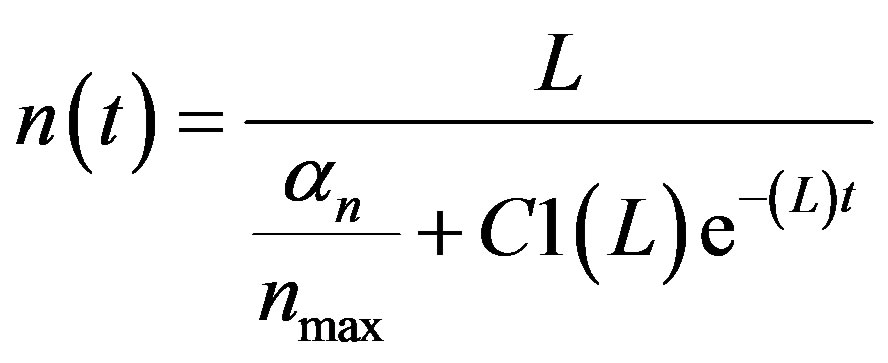 (A4)
(A4)
From Equation (A4), we can find the constant C1 can be obtained by substitute the initial condition. We get
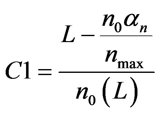 (A5)
(A5)
Substitute Equation (A5) in Equation (A4), the final solution is obtained.
 (A6)
(A6)
where 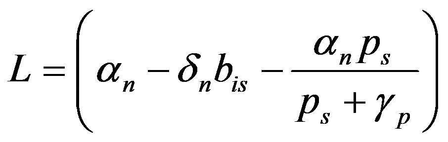 (A7)
(A7)
When , the above equation becomes
 (A8)
(A8)
Appendix B
Scilab/Matlab program to find the numerical solution of Equations (1)-(5).
function main1 options= odeset('RelTol',1e-6,'Stats','on');
Xo = [0.01;0;0;0;0];
tspan = [0,40];
tic
[t,X]= ode45(@TestFunction,tspan,Xo,options);
toc figure holdon plot(t, X(:,1))
%plot(t, X(:,2))
%plot(t, X(:,3))
%plot(t, X(:,4))
%plot(t, X(:,5))
return function [dx_dt]= TestFunction(t,x)
an=0.66;ar=0.01;ap=0.01;ab=0.01;
br=2.1;bp=0.66;
dn=0.91;db=0.5;
gp=0.14;gi=60;gr=1.8;
kr=10;kp=0.2;kb=100;nmax=1;
v=0.01;i1=1;
dx_dt(1)=(an*x(1)*(1-(x(1)/nmax)))-(dn*x(4)*x(1))-(an*x(1)*x(3)/(x(3)+gp));
dx_dt(2)=ar+(kr*(i1/(i1+gi)))-(br*x(2));
dx_dt(3)=ap+(kp*(1/(gr+(x(2)/(1+(kb*x(4)))))))-(x(3)*bp);
dx_dt(4)=(ab*x(1))-(x(3)*db*x(4));
dx_dt(5)=v*db*x(3)*x(4)*x(1);
dx_dt = dx_dt';