Engineering
Vol.6 No.9(2014), Article
ID:48511,7
pages
DOI:10.4236/eng.2014.69052
Empirical Model to Calculate the Thermodynamic Wet-Bulb Temperature of Moist Air
Melitón Estrada-Jaramillo1, Iván Vera-Romero1, José Martínez-Reyes1, Agustina Ortíz-Soriano2, Edgar Barajas-Ledesma1
1Trajectory of Energy Engineering, University of the Ciénega of Michoacán State, Sahuayo, México
2Trajectory of Educational Innovation, University of the Ciénega of Michoacán State, Sahuayo, México
Email: mestrada@ucienegam.edu.mx
Copyright © 2014 by authors and Scientific Research Publishing Inc.
This work is licensed under the Creative Commons Attribution International License (CC BY).
http://creativecommons.org/licenses/by/4.0/


Received 18 June 2014; revised 20 July 2014; accepted 30 July 2014
ABSTRACT
An equation model for calculating the adiabatic temperature of the wet-bulb thermometer has been obtained empirical fit through a meteorological database, specificly a trough relative humidity and air temperature. A comparison of the results of calculations with the use of this equation and from meteorological database was made. The model deducted of the comparison is valid for a dry bulb temperature range of 3˚C to 35˚C and for relative humidity percentage in a range of 7% to 97%. Normalized errors are less than 5.5%. It means a maximum variation of 0.55˚C from data. However, this variation from error represents only 3.6% of the data sample. The equation model was satisfactory.
Keywords:Wet-Bulb Temperature Equation, Dry-Bulb Temperature, Relative Humidity, Dry Solar Technologies, Humidified Gas Turbines

1. Introduction
The condensation and vaporization processes are important in different conventional and non-conventional systems of energy, using fossil fuel or renewable energies, and in systems applied to refrigeration, evaporation, air conditioning, humidification, condensation, dehumidification and airing. For example, as in [1] it shows a complete abstract about refrigeration for evaporation under different climate characteristics, and efficiency of several evaporative cooling equipments is indicated, through wet and dry bulb, and its relationship with mass and heat transference processes. These processes can be carried out using solar energy, through the use of different technologies as in [2] . In the industry of electrical production, they have application in the cogeneration systems, throughout compressed air to feed a gas turbine, and in cooling systems of incoming air to the turbines which allows output power increase, and improves thermal efficiency; these efficiencies are obtained through local climate conditions. The calculations began with determination of temperature of wet bulb ambient as in [3] . Also, they have application in the different gas turbine cycles as water injection cycles, steam injection cycles and evaporative cycles with humidification [4] [5] . Design and analysis of all these systems require knowledge of properties corresponding to dry air and steam water mixture from local environment. Calculus methodology of those properties from dry bulb temperature (Tdb), relative humidity (ϕ), local altitude (Z) is known and is shown by ASHRAE [6] . However, to determine thermodynamic wet bulb temperature(Twb), according to the methodology, a numerical implementation is necessary [7] -[11] .
In the present work, an equation to determine wet bulb temperature for mentioned conditions, is presented. It was obtained by processing numerical data of a Meteorological Station located in the region Ciénega of Chapala in Michoacán México, with latitude 20˚0'52.24''N and length 102˚44.37'37.11''W. During the numerical analysis 91,519 data were processed, for each of the variables involved, and they correspond to a typical local year.
2. Methodology
The considered variables for the analysis were dry bulb temperature and relative humidity, in ranges from 3˚C to 35˚C, and 7% to 97% respectively, with local altitude Z = 1526 m [12] . Wet bulb temperature was determined considering data equation and according to methodology described by ASHRAE, throughout a numerical implementation. Data were grouped as a function of relative humidity; the ranges consisted of 5 units, as it can be seen in Figure 1.
For each humidity range Twb vs Tdb were plotted and a linear adjusted equation was obtained, with general form: Twb = ATdb + B. Table 1 shows adjustment equations for each humidity range and the coefficients of determination.
Then, coefficients for A and B were correlated, for each humidity range considered (average of the range) as shown in Figure 2. Thus, Equation (1) was obtained and polynomial for coefficients A and B.
 (1)
(1)
In Equation (1), relative humidity is considered dimensionless, with Tdb and Twb given in ˚C. Adjusted coefficient values for each polynomial, are shown in Table2
3. Results and Discussion
Equation (1) has in its general form a linear behavior for dry bulb temperature. But coefficients Ai and Bi de-
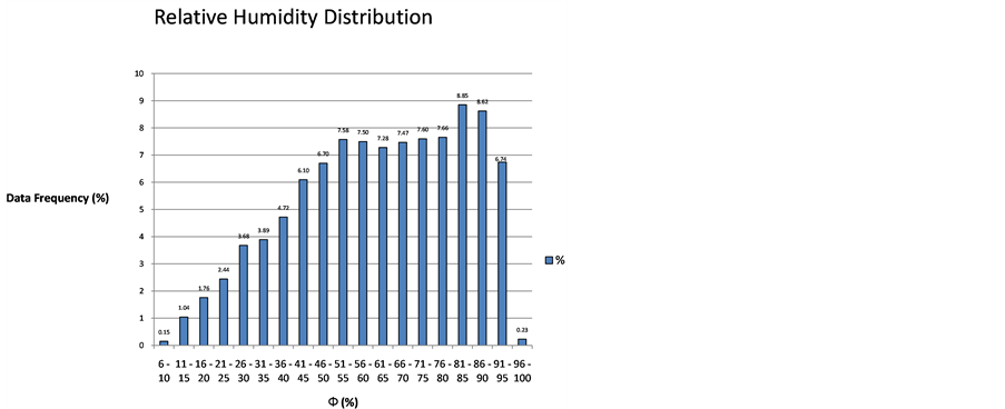
Figure 1. Percentage distribution for humidity ranges.
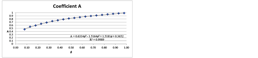
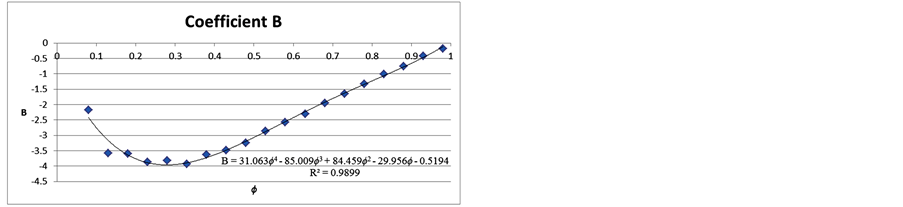
Figure 2. Polynomial coefficients for A and B with coefficients of determination.

Table 1. Adjustment equations from Twb and Tdb for each interval humidity.
Table 2. Fit coefficients for proposal equation.
pend on relative humidity, and they are 3th and 4th degree polynomials.
Figure 3 shows the correlation of Tdb, ϕ, Twb for data station and it is compared with the obtained values from Equation (1), for mentioned ranges, with acceptable fit.
In order to evaluate Equation (1), two errors are estimated: normalized error (En) and real error (Er). These are obtained from base data and with calculated data, according to the proposed equation. Normalized error evaluation was obtained using the following equation: . And real error using equation:
 .
.
Figure 4 shows the error between the proposed model and wet bulb temperature data from the meteorological station. The maximum normalized error is 5.4% (secondary vertical axis, En) and is equivalent to maximum variation of 0.6˚C as shown in the main vertical axis (Er). Absolute average error is 0.065% (En_av) about meteorological station, representing an average variation of a hundredth degree Celsius from real error (Er_av = 0.011˚C).
Also, Figure 4 shows that normalized error is present in a range of −6 and 3, and to estimate how this error impacts in base data, absolute frequencies were settled, from normalized error.
Table 3 shows absolute frequencies, this is to estimate the data quality from normalized error. This table shows an En range (Xj) according to Figure 4. Absolute frequency is determined by data selection and it is clear that between 1.0 and −1.0 a percentage of 96.4 of the obtained data are present.
Figure 5 shows data from Table 1 plotted, and 88,265 data are between 1.0 and −1.0, which indicates that the
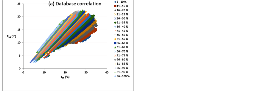

Figure 3. Comparison of Tdb, ϕ, Twb correlation of meteorological data (a); and from proposed model according to Table 1(b).
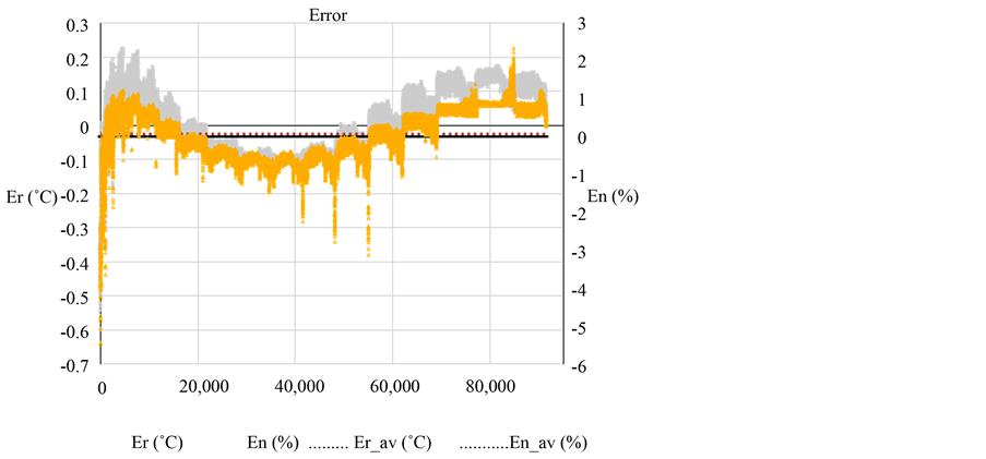
Figure 4. Comparison between real error and normalized error evaluated with data from meteorological station.
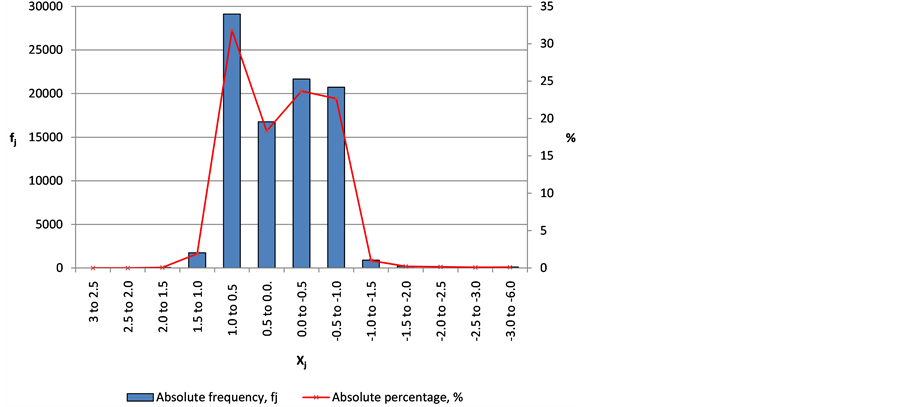
Table 3. Absolute frequency with its corresponding percentage to En data.
difference of real error and normalized error are in an acceptable value (only 3.6% of total data are out of 1.0 and −1.0).
4. Conclusion
A direct equation was obtained in order to predict wet bulb temperature, from relative humidity and dry bulb temperature. Methodology used to obtain the model, was in an empiric way, grouping relative humidity in ranges of 5 units, and for each range wet and dry bulb temperatures were correlated, obtaining a general linear adjust. Also, coefficients A and B were evaluated. Quality of generated data for the model was settled through error analysis. Normalized errors are less than 5.5%. It means a maximum variation of 0.55˚C from data. The normalized error applies only to 3.6% of the data considered in the present work. The model has an acceptable fit. It is valid for a range of temperature and relative humidity of 3˚C to 100˚C and 7% to 97% respectively. The pressure was calculated from the local altitude and the model behavior was not explored at different pressures. The equation obtained represents an important tool that facilitates the analysis and engineering calculations of various important energy processes.
References
- Xuan, Y.M., Xiao, F., Niu, X.F., Huang, X. and Wang, S.W. (2012) Research and Application of Evaporative Cooling in China: A Review (I)—Research. Renewable and Sustainable Energy Reviews, 16, 3535-3546.http://dx.doi.org/10.1016/j.rser.2012.01.052
- Saudagar, R.T., Ingole, P.R., Mohod, T.R. and Choube, A.M. (2013) A Review of Emerging Technologies for Solar Air Conditioner. International Journal of Innovative Research in Science, Engineering and Technology, 2, 2356-2359.
- Farzaneh, G.M. and Deymi, D.M. (2011) Effect of Various Inlet Air Cooling Methods on Gas Turbine Performance. Energy, 36, 1196-1205. http://dx.doi.org/10.1016/j.energy.2010.11.027
- Rydstrand, M.C., Westermark, M.O. and Bartlett, M.A. (2004) An Analysis of the Efficiency and Economy of Humidified Gas Turbines in District Heating Applications. Energy, 29, 1945-1961.http://dx.doi.org/10.1016/j.energy.2004.03.023
- Jonssona, M. and Yan, J. (2005) Humidified Gas Turbines—A Review of Proposed and Implemented Cycles. Energy, 30, 1013-1078. http://dx.doi.org/10.1016/j.energy.2004.08.005
- American Society of Heating, Refrigerating and Air-Conditioning Engineers (2001) ASHRAE Fundamentals Handbook (SI). Chapter 6. Psychrometrics. 6.1-6.17. Atlanta.
- Alliston, C.W. and Wolfe, S.A. (1973) Computation and Summary of Psychrometric Data from Dry Bulb and Dew Point Temperatures. Agricultural Metereology, 11, 169-176. http://dx.doi.org/10.1016/0002-1571(73)90061-7
- Wilhelm, L.R. (1976) Numerical Calculation of Psychrometric Properties in SI Units. Transactions of the ASAE (American Society of Agricultural Engineers), 19, 318-321. National Agricultural Library Catalog (AGRICOLA), Beltsville.
- Singh, A.K., Singh, H., Singh, S.P. and Sawhney, R.L. (2002) Numerical Calculation of Psychrometric Properties on a Calculator. Building and Environment, 37, 415-419. http://dx.doi.org/10.1016/S0360-1323(01)00032-4
- Wang, D.C., Fang, W. and Fon, D.S. (2002) Development of a Digital Psychrometric Calculator Using MATLAB. Acta Hort, 578, 339-344.
- Nelson, H.F. and Sauer, H.J. (2003) Thermodynamic Properties of Moist Air: -40 to 400°C. Proceedings of the 41st Aerospace Sciences Meeting and Exhibit, Reno Nevada, 6-9 January 2003, 1-11.
- Anguiano, J.C., Ruíz, J.C., Alcántar, J.R., Vizcaino, I.V. and González, I.A. (2006) Basic Climatological Statistics of Michoacán State (Period 1961-2003). Technical Book No. 3. INIFAP, México.
Nomenclature
 Fit Coefficients ASHRAE American Society of Heating, Refrigerating and Air-Conditioning Engineers En Normalized Error, % En_av Absolute Normalized Average Error Er Real Error, ˚C Er_av Real Average Error fj Absolute Frequency N North W West R2 Coefficient of Determination
 Temperature, ˚C Xj Range, Corresponding to En Values.
Z Local Altitude, m
Φ Relative humidity, %
ϕ Relative Humidity, Dimensionless
Subscript
db Dry bulb DB Database i Component i-th of fit Coefficients j Data from En
n Normalized r Real wb Wet bulb