Engineering
Vol. 5 No. 8 (2013) , Article ID: 35523 , 5 pages DOI:10.4236/eng.2013.58076
Comparisons of Oil Production Predicting Models
1School of Graduate of Southwest Petroleum University, Chengdu, China
2China Petroleum Engineering Construction Corporation, Beijing, China
3School of Science of Southwest Petroleum University, Chengdu, China
4Sichuan College of Architectural Technology, Deyang, China
5School of Petroleum Engineering Management of Southwest Petroleum University, Chengdu, China
Email: *tsinghua616@163.com
Copyright © 2013 Yishen Chen et al. This is an open access article distributed under the Creative Commons Attribution License, which permits unrestricted use, distribution, and reproduction in any medium, provided the original work is properly cited.
Received June 11, 2013; revised July 11, 2013; accepted July 18, 2013
Keywords: Oil Field; Oil Production; Model; Predicting Accuracy
ABSTRACT
Feasibility of oil production predicting results influences the annual planning and long-term field development plan of oil field, so the selection of predicting models plays a core role. In this paper, three different predicting models are introduced, they are neural network model, support vector machine model and GM (1, 1) model. By using these three different models to predict the oil production in XINJIANG oilfield in China, advantages and disadvantages of these models have been discussed. The predicting results show: the fitting accuracy by the neural network model or by the support vector machine model is higher than GM (1, 1) model, the prediction error is smaller than 10%, so neural network model and support vector machine model can be used to short-term forecast of oil production; predicting accuracy by GM (1, 1) model is not good, but the curve trend with GM (1, 1) model is consistent with the downward trend in oil production, so GM (1, 1) predicting model can be used to long-term prediction of oil production.
1. Introduction
Oil production prediction is very important in the oilfield development; study on oil production predicting method is a key topic of petroleum science. At present, there are four kinds of predicting methods [1-6] with physical meanings: Empirical formula such as Arps method, Hubbert model, water-flood decline curve method; Hydrodynamic model based on fluid mechanics model; Material balance equation model; Numerical reservoir simulation model. Besides the above mentioned four methods, there is a typical type of prediction model related to modern optimization, this model type is composed of GM (1, 1) model, neural network model, support vector machine model, etc. Oil field development system is a complex multi variables non-linear dynamical systems, different predicting model has different characteristics like predicting accuracy. Neural network model and support vector machine model are two effective methods to solve multi nonlinear mapping problem. At present they are used in many disciplines, even in the oil production prediction. In this paper, neural network model and support vector machine model have been used to predict the oil production of XINJIANG oil field, and good predicting results have been achieved. Meanwhile, GM (1, 1) model has also been used to predict oil production. Predicting result shows that this model is adaptable to the case which lacks data and hard to establishes model with probabilistic method.
2. Predicting Model
2.1. Neural Network Predicting Model
At present, in the application of artificial neural networks (ANN) [7,8], most of them are back propagation (BP) ANN and their variations. It has been proved that BP neural network can approximate any multivariate continuous function. Kolmogorov rule guaranteed that any continuous function or mapping can be achieved by a 3-layer ANN.
3-layer BP ANN is used to establish the ANN model with prediction function. The first layer of BP-ANN is input layer, the second layer of it is middle layer, and the third layer of it is the output layer, see Figure 1.

Figure 1. BP neural network structure.
Network Simulation
Assume N-samples (input-output data samples) are used during the training process:
The input variables are  , the output variables are
 . For the k-sample
 , let.
  be input mode vector;
  be the expectation output vector;
  be the middle layer input vector;
  be the output unit vector of middle layer;
  be the input vector of output layer;
  be the output vector of output layer;
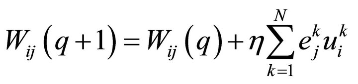
  be the connection weights from input layer to middle layer;
  be the connection weights from middle layer to output layer;
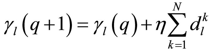
  be the threshold value of middle layer;
  be the threshold value of output layer;
  is the learning rate.
Let the response function of ANN  be Sigmoidtype function:
The input and output values of each neural unit satisfy the following relationship:
Middle layer:
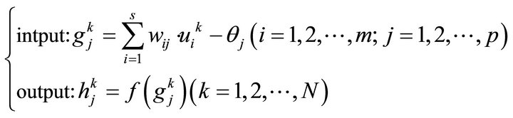
(1)
Output layer:
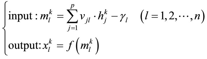 (2)
(2)
After training of N samples, the network error is:
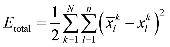 .
.
Error of output layer unit:
 (3)
(3)
Error of middle layer unit:
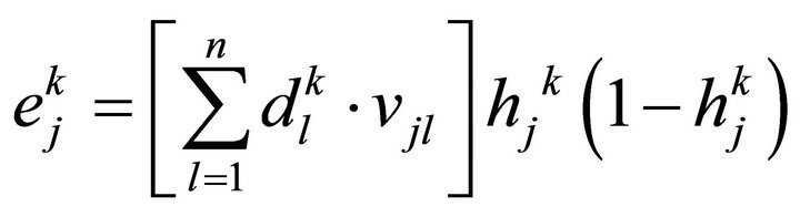 (4)
(4)
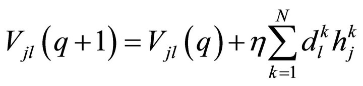
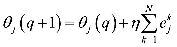
The connection weights  and the threshold value
  can be modified by the output layer error
  and output value of middle layer unit
 :
:
 (5)
(5)
 (6)
(6)
The connection weights  and the threshold value
  can be modified by the middle layer error
  and input value of input layer
 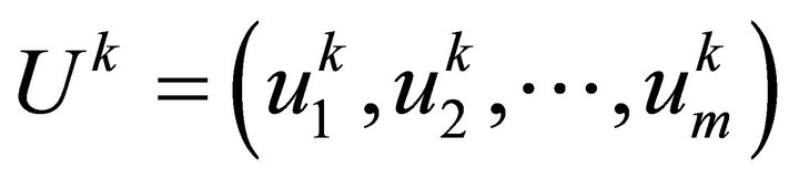 :
:
 (7)
(7)
 (8)
(8)
Repeat the above-mentioned learning mode, until the network converges to a given error range.
2.2. Support Vector Regression(SVR) Predicting Model
SVR [9-11] is an effective method to solve the regression problem. This regression problem can be described in mathematics:
Given training set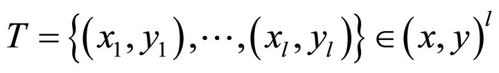 , where
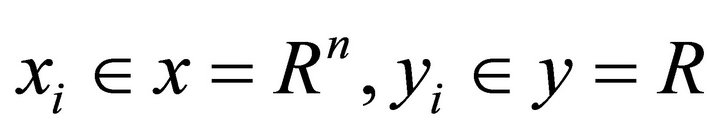 ,
, . The training set is composed of independent and identically distributed sample points following certain probability distribution
 . After giving loss function
 , the regression function
 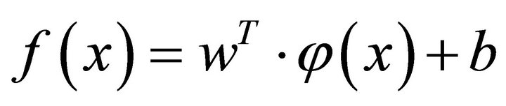 will be found to make the expected risk
 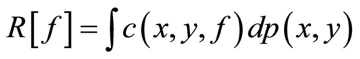 reach its minimum value, where
  is the nonlinear mapping, it maps the data
 into a high dimensional feature space;
  and
and  are weight vector and bias value, separately.
If we denote the regression problem by minimum risk problem with the loss function 
 , then the basic rule of SVR method is established: by introducing kernel function
  into the nonlinear mapping, the nonlinear regression problem in lowdimensional input space transformed into a linear regression problem in high dimensional feature space and the key is to solve the parameter
  and
and  in the regression function. Hence, the basic rule of SVR in solving regression problem is to solve an optimal problem with the following form:
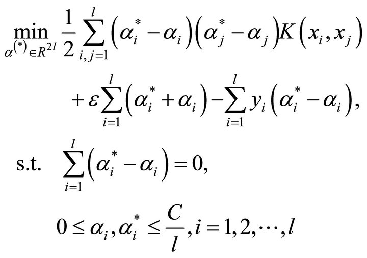 (9)
(9)
where 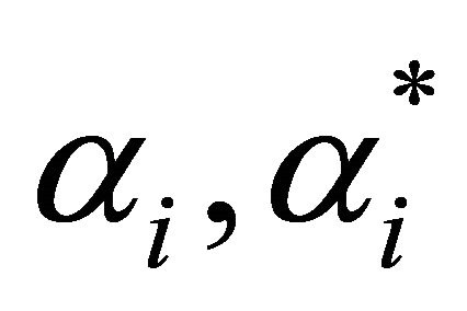 are Lagrange multipliers;
 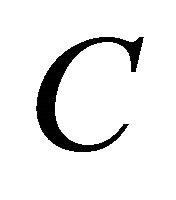 is a constant, called penalty factor;
 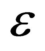 is a given positive value, it is a maximum error of regression.
By solving Equation (9) gives the optimal Lagrange multipliers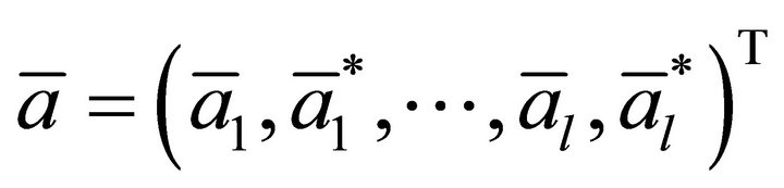 , and then gives regression function when the expected risk
  gets its minimum:
 (10)
(10)
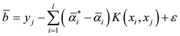
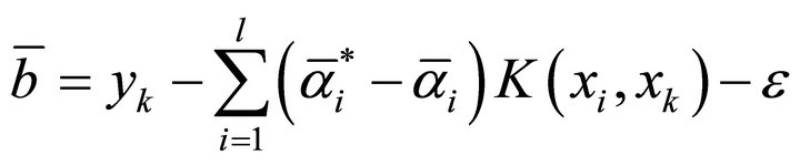
where the sample satisfied  is the support vector;
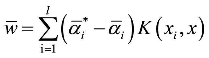 .
.
Select  or
or  in interval
 ;
;
If  is selected, then
If  is selected, then
when solving regression problem, the proper kernel function can be selected to SVR training. Introducing sample factor vector  and predictor vector
  into Equation (10) after training gives the prediction result.
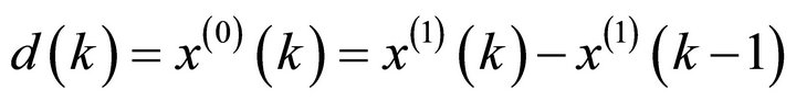
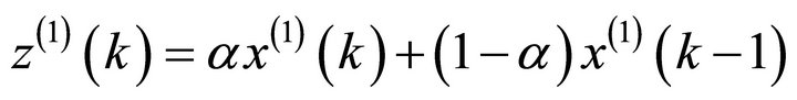
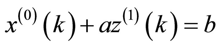
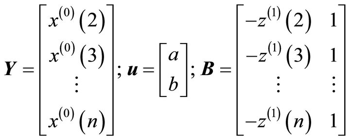
2.3. GM (1,1) Predicting Model
The Let  be initial data series, its 1-AGO data series is
 where
where  denote the grey derivative of
  by:
by:
Let 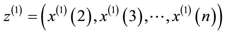 be the generated data series of
 , then
Hence, denote the gray differential equation model of GM (1, 1) [12,13] by:
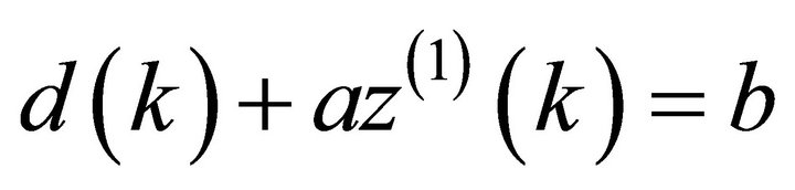
It is,
 (11)
(11)
In Equation (11)  is the grey derivative,
  is the developing coefficient,
  is the albino background value,
  is the grey functional variable.
Introducing  into Equation (13) gives

Let
Then GM (1, 1) model can be expressed as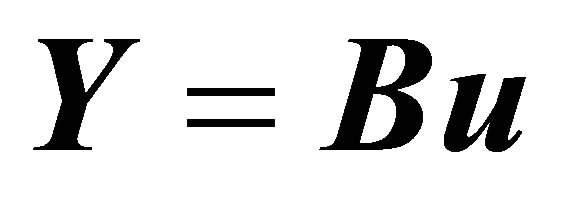 , now the question comes down to find the value of
 .
.
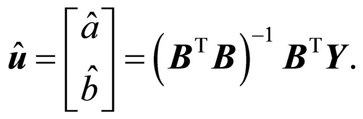
Introducing least square method to solve the estimating value:
In Equation (13), if  is continuous variables when
 , then
  is a function of time
 , it is
 , so the derivative of
  become
 and the derivative of albino background value
 becomes
 . Hence, the grey differential equation becomes:
 (12)
(12)
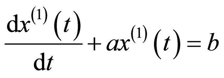
Equation (12) is the albino type of GM (1, 1) model. Given initial value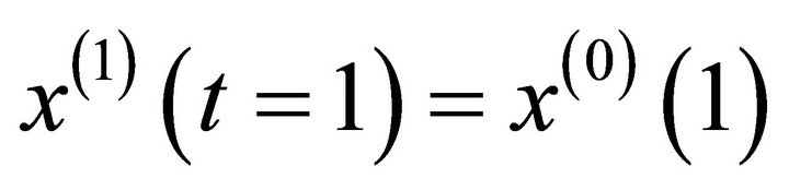 , the solution of Equation (12) becomes:
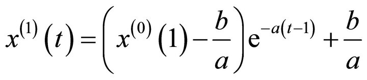 .
.
3. Applications and Discussions
Given the initial oil production data (from 1958 to 2012) of certain oilfield block in China, then the above-mentioned three method can be used to predict the oil production of different oilfield block (A1, A2, A3). After using the above-mentioned three different predicting model gives Figures 2-4.
In Figures 2-4, the black circle means the real oil production, the green curve is the predicting curve with ANN model, the red curve is the predicting curve with SVR model, the blue curve is the predicting curve with GM (1, 1) model. Figures 2-4 show the predicting accuracy with ANN model and SVR model is higher than

Figure 2. comparison of oil production prediction value with different method in block-A1.
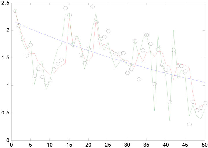
Figure 3. comparison of oil production prediction value with different method in block-A2.
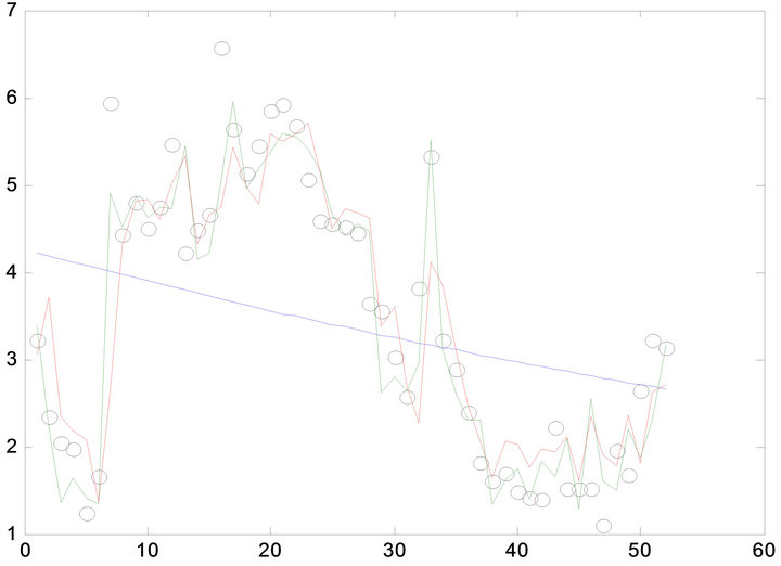
Figure 4. comparison of oil production prediction value with different method in block-A3.
the GM (1, 1) model, the maximum relative error is less than 10%, ANN model and SVR model can be used to short term prediction. However, the GM (1, 1) model predicts the overall trend in oil production decline; it can be used to middle-long term oil production prediction.
4. Conclusions
Prediction with ANN model and SVR model can comply with the actual oilfield production dynamics, the prediction errors of them are less than 10%. However, they are learning type of model; much data is needed to complete the prediction, so they are only suitable for the short term prediction;
Although the prediction accuracy with GM (1, 1) model is low, still the prediction result fits with the overall downward trend of oil production, so it can be used as a reference for long-term prediction.
REFERENCES
- B. Y. Ji, “Overview of Oilfield Development Indicators Forecasting Methods,” Petroleum Geology and Oilfield Development in Daqing, Vol. 18, No. 2, 1999, pp. 19-22.
- J. G. Hu, Y. Q. Chen and S. Z. Zhang, “A New Model Using for Prediction of Oil-Gas Field Production,” Acta Petrolei Sinica, Vol. 16, No. 1, 1995, pp. 79-86.
- G. Chen and X. L. Yang, “An Examination into Prediction Methods Based on Reservoir Performance Analyses,” China Offshore Oil and Gas (Geology), Vol. 16, No. 4, 2002, pp. 254-259.
- Y. Q. Chen and Q. F. Zhao, “A Combined Method of Weibull Model and Water Drive Curve of B Type,” Xinjiang Petroleum Geology, Vol. 21, No. 5, 2000, pp. 405- 407.
- Y. Q. Chen, J. G. Hu and D. J. Zhang, “Deduction of Logistic Model and Auto Regression Methods,” Xinjiang Petroleum Geology, Vol. 17, No. 2, 1996, pp. 150-155.
- P. Yue, X. F. Chen, L. G. Cui, et al., “Suggestion Solution of Weng’s Model and Logistic Model in Production Research,” Journal of Oil and Gas Technology, Vol. 31, No. 4, 2009, pp. 277-279.
- B. Yang, “Applied Neural Network in Oil Well Logging,” Petroleum Industry Press, Beijing, 2005.
- X. G. Wu and J. L. Ge, “Oil Production Forecast with ANN Method,” Petroleum Exploration and Development, Vol. 21, No. 3, 1994, pp. 31-42.
- C. H. Zhang, “Optimization Problems in Support Vector Machines,” China Agricultural University Doctoral Dissertation, Vol. 5, 2004, pp. 36-39.
- Z. H. Feng and J. M. Yang, “Practical Selection of Support Vector Machine Parameters for SVM Regression,” Mechanical Engineering and Automation, Vol. 3, 2007, pp. 17-18.
- K. Ito and R. Nakano, “Optimizing Support Vector Regression Hyperparameters Based on Cross-Validation,” Proceedings of the International Joint Conference on Neural Networks, Vol. 3, 2003, pp. 2077-2082.
- J. M. Yao, B. S. Yu, et al., “Application of the Improved GM Model to Oil Production Forecasting of Tarim Basin,” Petroleum Geology and Oilfield Development in Daqing, Vol. 26, No. 1, 2007, pp. 92-96.
- M. F. Chen and Z. X. Lang, “Oil Production Forecasting with Modified Functional Simulation Model,” Xinjiang Petroleum Geology, Vol. 24, No. 3, 2003, pp. 246-248.
NOTES
*Corresponding author.