Engineering
Vol.5 No.6(2013), Article ID:33265,8 pages DOI:10.4236/eng.2013.56065
Finite Element Modeling of Seismic Response of Field Fabricated Liquefied Natural Gas (LNG) Spherical Storage Vessels
Department of Mechanical Engineering, University of Ibadan, Ibadan, Nigeria
Email: deleadeyefa@yahoo.com
Copyright © 2013 Oludele Adeyefa, Oluleke Oluwole. This is an open access article distributed under the Creative Commons Attribution License, which permits unrestricted use, distribution, and reproduction in any medium, provided the original work is properly cited.
Received April 5, 2013; revised May 6, 2013; accepted May 16, 2013
Keywords: FEM; LNG; Seismic; FORTRAN; Newmark; UBC; ASME
ABSTRACT
All real physical structures behave dynamically when subjected to loads or displacements. This research paper, therefore, presents seismic response of field fabricated liquefied natural gas spherical storage vessels using finite element analysis. The seismic analysis procedure used represents a practical approach in quantifying the response of spherical storage vessel with its content when it is subjected to seismic loading. In the finite element method approach, six degrees of freedom per node is used for legs/column of the spherical storage tanks. Lumped mass procedure is employed to determine system mass matrix of the structure. Computer programme code is developed for the resulting matrix equation form finite element analysis of the structure using FORTRAN 90 programming language. The modeling of the seismic load utilizes the ground acceleration curve of a site. From the results of the modal analysis, the system is uncoupled thereby gives way to the application of Newmark’s method. Newmark’s method as one of the widely used time-step approach for the seismic response is applied. The developed programme coding is validated with analytical results (P > 0.5). It shows that the approach in this research work can be successfully used in determine the stability of large spherical storage vessels against seismic loadings when base acceleration spectral of the site are known. This approach gives better results than the static-force approach which gives conservative results. While the approach used in this research treats seismic loads as time event, static-force approach assumed that the full ground force due to seismic motion is applied instantaneously.
1. Introduction
In more and more engineering situations today, it is necessary to obtain approximate numerical solutions to problems rather than exact closed-form solutions. It is discovered that many of the engineering problems faced by engineers in today’s world present no simple analytical solutions. Though, design engineer may have been able to write down the governing equations and boundary conditions for the problem, yet he sees immediately that no simple analytical solution can be found. The difficulty in these types of engineering problems lies in the fact that either the geometry or some other feature of the problem is irregular or “arbitrary”. Analytical solutions to problems of this type seldom exist; yet these are the kinds of problems that design engineers are called upon to solve.
The resourcefulness of the analyst usually comes to the rescue and provides several alternatives to overcome this dilemma. One possibility is to simplify the difficulties and reduce the problem to one that can be handled. Sometimes this procedure works; but, more often than not, it leads to serious inaccuracies or wrong answers. Now that high-speed computers are widely available, a more viable alternative is to retain the complexities of the problem and find an approximate numerical solution.
Finite element method is one the widely used approximate numerical method and its model of a problem gives a piecewise approximation to the governing equations. The basic premise of the finite element method is that a solution region can be analytically modeled or approximated by replacing it with an assemblage of discrete elements. Since these elements can be put together in a variety of ways, they can be used to represent exceedingly complex shapes. Though, the finite element method can be used to solve a very large number of complex problems, there are still some practical engineering problems that are difficult to address because we lack an adequate theory of failure, or because we lack appropriate material data. This is not a finite element problem, but is of serious concern to any engineer who wants to supplant testing with analysis. The use of analysis usually permits faster design turnaround, the exploration of widely varying environments, and the use of optimization tools.
The seismic analysis procedures outline in Universal Building Code (UBC) is static-force procedures, which assume that the entire seismic force due to ground motion is applied instantaneously. This assumption is conservative but greatly simplifies the calculation procedures. In reality earth quakes are time-dependent events and the full force is not realized instantaneously. The UBC allows, and in some cases requires, that a dynamic analysis be performed in lieu of the static—force method. Although much more sophisticated, often the seismic loadings are reduced significantly.
2. Finite Element Methodology
The most common and effective approach for seismic analysis of linear structural systems is the mode superposition method. After a set of orthogonal vectors have been evaluated, this method reduces the large set of global equilibrium equations to a relatively small number of uncoupled second order differential equations. The numerical solution of those equations involves greatly reduced computational time.
2.1. Model Assumptions
Below are the assumptions made in the model in this research work:
1) The storage tank is full of water, hydrotest, for the worst case scenario. This gives maximum compressive load/force per leg support.
2) In determining the system mass matrix, lumped sum mass matrix is employed.
3) The only externally applied load/force is the weight of the content (tank full of water) and shell. Externally applied force on each of the leg is the sum of the weight of content (tank full of water) and shell divided by the number of legs. While there is base acceleration applied to the support due to seismic effect Figure 1.
4) Seismic effect on one of the storage tank support legs is representative of the effect of seismic load on the entire storage tank structure. If one of the legs fails due to seismic load, the entire structure fails Figure 2.
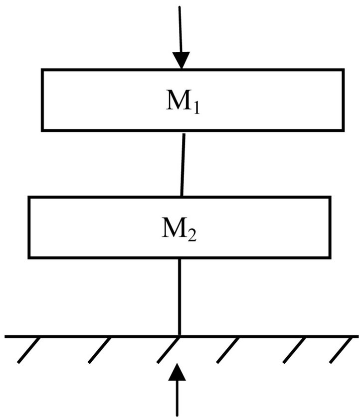
Figure 1. Typical vibration model with compressive force and earth/support motion.

Figure 2. Showing section of spherical tank with leg support.
2.2. Dynamic Equilibrium
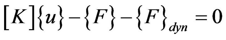
Taking into account the equivalent static force, the general equations of equilibrium for a structure is as follows
 (1)
(1)
where {F} is the force vector representing the external applied forces as a function of time. {F}dyn, is the assembled force vector for the complete structure due to inertia and damping forces. [K] is the system static stiffness matrix and {u} is nodal displacement.
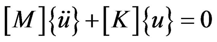
For many structural systems, the approximation of linear structural behaviour is made to convert the physiccal equilibrium statement, Equation (1), to the following set of second-order, linear, differential equations, general equation of motion
 (2)
(2)
where M is the mass matrix (lumped or consistent), C is a viscous damping matrix (which is normally selected to approximate energy dissipation in the real structure) and K is the static stiffness matrix for the system of structural elements. The time-dependent vectors,  ,
,  and u are node accelerations, velocities and displacements respectively.
2.3. System Stiffness Matrix
To determine the stiffness matrix for the beam-column support of spherical storage vessels. It is assumed that a typical member leg can be thought of a 3-D space frame having four actions: two bending actions, a twisting action, and an axial action. Thus, the displacement of each node is described by three translational and three rotational components of displacement, giving six degrees of freedom at each unrestrained node. Corresponding to these degrees of freedom are six nodal loads. The notations use for the displacement and force vectors at each node are, respectively,
 (3a)
(3a)
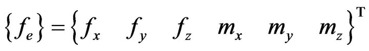 (3b)
(3b)
On the local level, for each member, the forces are related to the displacements by the partitioned matrices
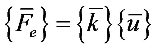 (4)
(4)
 (5)
(5)
where


 ,
, 
E is the elastic modulus, G is the modulus of rigidity, Le is the length of beam-column element, Ix, Iy, and Iz are the second moment of inertia about x, y, and z respectively.
2.4. System Mass Matrix
It is useful to realize that using lumped mass method to generate the system mass matrix, the methodology does not involve derivatives of the shape functions. We can therefore be more lax about the choice of shape function for the determination of system mass matrix than for the stiffness matrix. In many applications, it is preferable to use a lumped mass (and damping) approximation where the only nonzero terms are on the diagonal. The simplest mass model is to consider only the ger translational inertias, which are obtained simply by dividing the total mass by the number of nodes and placing this value of mass at the node. Thus, the diagonal terms for the 3-D frame can be given as
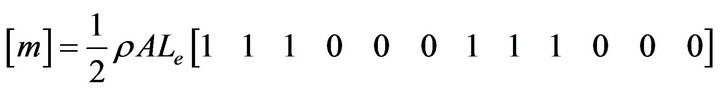 (6)
(6)
where ρ is material density of beam element, A is the beam-column cross sectional area and Le is the length of beam-column and [M] is the mass matrix.
These neglect the rotational inertias of the flexural actions. Generally, many researchers in the field of finite element methods had proved that the contributions of the rotational inertia of the flexural actions to the system mass matrix are negligible and matrix Equation (6) above is quite accurate especially when the elements are small. There is, however, a very important circumstance when a zero diagonal mass is unacceptable and reasonable nonzero values are needed. In the present research, a zero diagonal mass is unacceptable because this leads to computer programme error when applying Newmark’s method for the seismic response analysis. Therefore, Equation (6) is then modified to give equation below with non-zero diagonal.
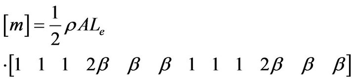 (7)
(7)
where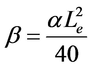 .
.
where ![]() is typically taken as unity. This scheme has the merit of correctly giving the translational inertias. Therefore, estimate the effective length L ≈ √A/π as basically the radius of a disk of the same area as the triangle. Again, α is typically taken as unity.
is typically taken as unity. This scheme has the merit of correctly giving the translational inertias. Therefore, estimate the effective length L ≈ √A/π as basically the radius of a disk of the same area as the triangle. Again, α is typically taken as unity.
2.5. Free Undamped Vibration Mode
The structure is not excited externally in free vibration mode i.e. no force or support motion acts on it. So, under the condition of free motion, dynamic analysis can be carried out and the important properties like natural frequencies and mode shapes corresponding to the natural frequency can be obtained. Since free vibration mode is considered, the structure is not under the influence of any external force. Hence, the force and damping force vectors in stiffness equations are taken as zero.
By taking the above condition into consideration, the stiffness equation can be represented as,
 (8)
(8)
Thus  (9)
(9)
substituting Equation (9) into Equation (8) gives
 (10)
(10)
This is linear eigenvalue problem whose solutions, when arranged in order of magnitude of the eigenvalues, are approximation to the corresponding natural frequencies and normal modes of the vibration of the system. To convert the generalized eigenvalue problem to the standard form, the following steps need to be taken:
The general equation is written as
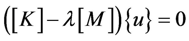 (11)
(11)
Rearranging Equation (11) gives
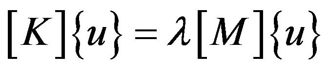 (11a)
(11a)
or
 (11b)
(11b)
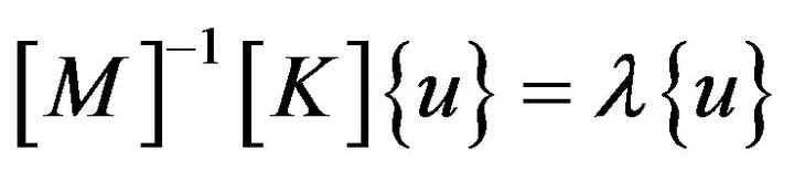
or
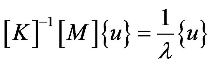 (11c)
(11c)
Equation (11c) may be rewritten as
 (12)
(12)
where [I] is an identity matrix The only problem with Equation (12) is that although [K] and [M] are symmetric, the product [K]–1[M] is generally not symmetric. To preserve symmetry, the Cholesky’s method may be used [1]. The Cholesky method decomposes a square, symmetric matrix to the product of an upper triangular matrix and the transpose of the upper triangular matrix. Applying the Cholesky decomposition to the matrix [K] gives
 (13)
(13)
Substituting Equation (13) into (12) and converting it into the standard form gives (Griffiths and Smith, 1991)
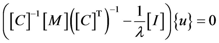 (14)
(14)
Equation (14) is in the form of a standard eigenvalue problem. It can be expressed more closely to Equation (11) if it is rewritten as
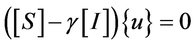 (15)
(15)
where  and
and 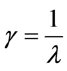
Since the matrices in eigenvalue problem often become very large, the matrices may be converted to a simpler form using Householder’s method before solving for the eigenvalues [1]. Householder’s method converts a symmetric matrix into a tridiagonal matrix. A tridiagonal matrix has non-zero elements only on the diagonal plus or minus one column [2]. Solutions are obtained using FORTRAN 90 programming language. The output of the program consists of the natural frequencies of the system with the corresponding mode shapes.
Since the matrices in eigenvalue problem often become very large, the matrices may be converted to a simpler form using Householder’s method before solving for the eigenvalues [1]. Householder’s method converts a symmetric matrix into a tridiagonal matrix. A tridiagonal matrix has non-zero elements only on the diagonal plus or minus one column [2]. Solutions are obtained using FORTRAN 90 programming language. The output of the program consists of the natural frequencies of the system with the corresponding mode shapes.
2.6. Transformation of Modal Equation
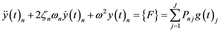
The dynamic force equilibrium Equation (2) can be rewritten in the following form as a set of N second order differential equations:
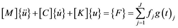 (16)
(16)
All possible types of time-dependent loading, including wind, wave and seismic, can be represented by a sum of “J” space vectors fj, which are not a function of time, and J time functions g(t)j. The number of dynamic degrees of freedom is equal to the number of lumped masses in the system.
The fundamental mathematical method that is used to solve Equation (16) is the separation of variables. This approach assumes the solution can be expressed in the following form:
 (17a)
(17a)
where  is an N by N matrix containing N spatial vectors that are not a function of time, and Y(t) is vector containing N functions of time.
From Equation (17a), it follows that:
 (17b)
(17b)
 (17c)
(17c)
Before solution, it is require that the space functions satisfy the following mass and stiffness orthogonality conditions:
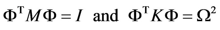 (18)
(18)
where I is a diagonal unit matrix and Ω2 is a diagonal matrix in which the diagonal terms are . The term
  has the units of radian per second.
After substitution of Equations (17) into Equation (16) and the pre-multiplication by , the following matrix of N equations is produced:
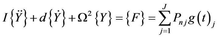 (19)
(19)
For three-dimensional seismic motion, this equation can be written as:
where  and are defined as the modal participation factors for load function j. The term Pnj is associated with the nth mode. There is one set of “N” modal participation factors for each spatial load condition fj. For all real structures, the “N by N” matrix is not diagonal; however, to uncouple the modal equations, it is necessary to assume classical damping where there is no coupling between modes. Therefore, the diagonal terms of the modal damping are defined by:
 (20)
(20)
where  is defined as the ratio of the damping in mode n to the critical damping of the mode [3]. A typical uncoupled modal equation for linear structural systems is of the following form:
 (21)
(21)
For three-dimensional seismic motion, this equation can be written as:
 (22)
(22)
where the three-directional modal participation factors, or in this case seismic excitation factors, are defined by  in which j is equal to x, y, or z and n is equal to the mode number.
By examining Equation (22) above, the damping term constant can be written as
 (23)
(23)
It has been shown that damping ratio of a structure is proportional to the structural stiffness. Therefore, this is then adopted in the present work and Equation (23) then becomes
 (24)
(24)
where  is the mode damping ratio.
2.7. Step by Step Numerical Integration Procedure
The step by step analysis is based on the powerful iterative technique developed by [4] known as Newmark’s  parameter method. The acceleration at the end of a time step is estimated, and the velocity and displacement are then calculated by
 (25)
(25)
![]() ,
,  , and
, and  represent the displacement, velocity, and acceleration of any point. The suffixes i and i + 1 representing the ends of the time intervals i and i + 1. The above expressions are substituted in the general equations of motion and a new estimate for the acceleration at the end of the time step i + 1 is determined. The process is repeated until successive values of the acceleration agree within a specified tolerance.
The parameter β in the Newmark’s equation governs the influence of the acceleration at the end of the time interval i + 1 on i + 1 the displacement at that instant. Furthermore, the value selected for β determines the variation of the acceleration during the interval Δt from i to i + 1, the method becomes a linear acceleration assumption [4]. A β value of 1/4 represents a constant acceleration throughout the interval and β = 1/8 may be interpreted as a step function having acceleration  over the first half of the time interval and u through the last half [4].
2.8. Participating Mass Ratio
This requirement is based on a unit base acceleration in a particular direction and calculating the base shear due to that load. The steady state solution for this case involves no damping or elastic forces; therefore, the modal response equations for a unit base acceleration in the x-direction can be written as:
 (26)
(26)
The node point inertia forces in the x-direction for that mode are by definition:
 (27)
(27)
The resisting base shear in the x-direction for mode n is the sum of all node point x forces. Or:
 (28)
(28)
The total base shear in the x-direction, including N modes, will be:
 (29)
(29)
For a unit base acceleration in any direction, the exact base shear must be equal to the sum of all mass components in that direction. Therefore, the participating mass ratio is defined as the participating mass divided by the total mass in that direction. Or:
 (30a)
(30a)
 (30b)
(30b)
 (30c)
(30c)
An examination of values giving by the factors in Equations (30) gives design engineer an indication of the value of the base shear associated with each mode. The angle with respect to the x-axis of the base shear associated with the first mode is given by:
 (31)
(31)
3. Seismic Response Analysis
Case 1: To validate the computer program developed, modal analysis is performed on a 2-degree of freedom structural system subjected to free undamped vibration with the following characteristics and the results are compared with the analytical method.
 , K=
, K=
Case 2:
Spherical pressure vessel leg support with the characteristics below is subjected to the seismic loading. The leg column is carbon steel, cold hollow circular pipe of outside diameter 323.9mm. The seismic loading in this model is base acceleration of Table 1.
Compressive vertical Load/force per leg (N) = 3465.0;
Moment of inertia about x-axis, Ix (m4) =28600 × 10−8;
Moment of inertia about y-axis, Iy (m4) =14300 × 10−8;
Moment of inertia about z-axis, Iz (m4) =14300 × 10−8;
Length of the support (m) =2.0;
Modulus of Elasticity, E (N/m2) =206.8 × 10⁹;
Poisson Ratio, v = 0.3;
Modulus of Rigidity, G (N/m2) = E/(2(1 + v));
Material Density (Kg/m3) = 7850;
Structural Damping proportional constant = 0.5.
4. Results and Discussions
The results of the Case 1 in Table 2 show that the FORTRAN coding developed in this research give better results of the natural frequency of free undamped vibration considered. In case two considered, Figure 3 gives the variation of natural frequencies against for different modes. Mode 7 gives highest natural frequency of value of over 4500 Hz while the least of all is mode 1 which gives natural frequency with value of zero Hz. Figures 3-6 give relative response of the second mode of vibration for acceleration, velocity and displacement.
In the computer simulation for the Case 2, the same value of damping ratio is assumed for all modes. The structural system under consideration has the same value for the damping constant in all modes. Also, the results show above for the case two simulation considered seismic effect in one direction alone—the vertical direction. In reality, the effects of base acceleration in different directions at the site on the structural system have to be considered and superimposed. By doing this, the design
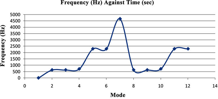
Figure 3. Showing frequency (Hz) against mode.
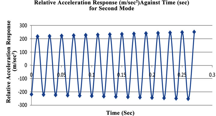
Figure 4. Showing relative acceleration response of second mode.

Figure 5. Showing relative velocity response of second mode.

Table 1. Showing typical earthquake ground acceleration with time.
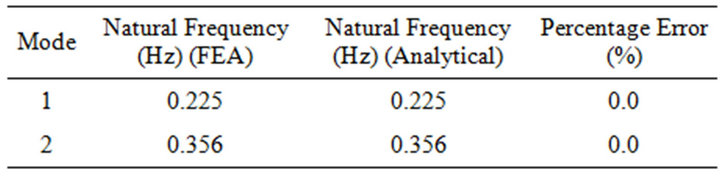
Table 2. Comparing FEA and analytical solutions.
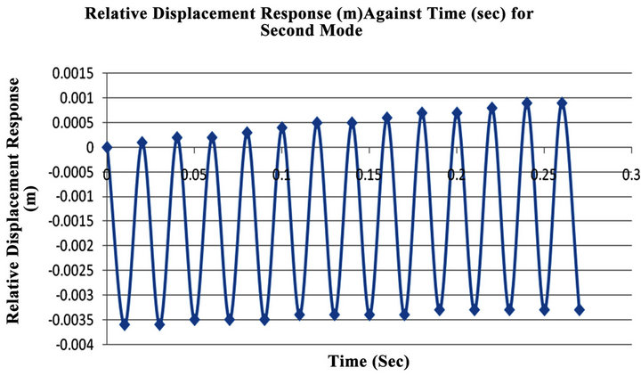
Figure 6. Showing relative displacement response of second mode.
engineer will be able to have better understating of the behavioral or response pattern of the structure to the seismic loading.
5. Conclusions and Recommendations
The use of finite element method in the seismic response analysis of field fabricated spherical pressure vessels cannot be over emphasized. This is also in line with the recommendation from UBC which allows design engineer to use other method such as finite element method in carrying out the seismic response of a structure. This is because; it is believed that static-force used by UBC code is conservative, and to get accurate response of any structure subjecting to seismic load the use of finite element analysis is desirable.
While it is noted that in ASME code section VIII Div 1, recommendation is made to consider other loads apart from internal and external pressures. Such other loads are wind, local and seismic yet it silent on procedures for determining the effects of such loads on pressure vessels. The decision, therefore, lies in the hands of design engineer to use any suitable method available at his disposal in analyzing effects of such loads on pressure vessels. One of such methods available to design engineers is finite element method. If this method is properly applied, it will give sound and safe design.
This research work has shed light on the methodology of applying finite element method to seismic response analysis of field fabricated spherical pressure vessels. The seismic analysis procedure used represents a practical approach in quantifying the response of spherical storage vessel with its content when it is subjected to seismic loading.
The result shows that the approach in this research work can be successfully used in determine the stability of large spherical storage vessels against seismic loadings when base acceleration spectral of the site is known. This approach gives better results than the static-force approach which gives conservative results.
REFERENCES
- D. V. Griffiths and I. M. Smith, “Numerical Methods for Engineers,” Blackwell Scientific Publications, London, 1991.
- W. H. Press, “Numerical Recipes in C: The Art of Scientific Computing,” Cambridge University Press, Cambridge, 1992.
- L. W. Edward, “Three-Dimensional Static and Dynamic Analysis of Structures,” A Physical Approach with Emphasis on Earthquake Engineering, Computers and Structures Inc., Berkeley, 2002.
- N. M. Newmark, “A Method of Computation for Structural Dynamics,” ASCE Journal of the Engineering Mechanics Division, Vol. 85, 1959, pp. 67-94.