Intelligent Control and Automation
Vol.4 No.1(2013), Article ID:27700,7 pages DOI:10.4236/ica.2013.41002
Sensor Fusion with Square-Root Cubature Information Filtering
Ford Motor Company of Canada Ltd., Windsor, ON, Canada
Email: haran@ieee.org
Received August 8, 2012; revised September 7, 2012; accepted September 14, 2012
Keywords: Cubature Kalman Filter; Information Filter; Multi-Sensor Fusion; Square-Root Filtering
ABSTRACT
This paper derives a square-root information-type filtering algorithm for nonlinear multi-sensor fusion problems using the cubature Kalman filter theory. The resulting filter is called the square-root cubature Information filter (SCIF). The SCIF propagates the square-root information matrices derived from numerically stable matrix operations and is therefore numerically robust. The SCIF is applied to a highly maneuvering target tracking problem in a distributed sensor network with feedback. The SCIF’s performance is finally compared with the regular cubature information filter and the traditional extended information filter. The results, presented herein, indicate that the SCIF is the most reliable of all three filters and yields a more accurate estimate than the extended information filter.
1. Introduction
Sensor fusion is generally defined as the use of techniques that combine data from multiple sensors such that the resulting information is more accurate and more reliable than that from a single sensor. Sensor fusion techniques are widely used in many applications such as mobile robot navigation, surveillance, air-traffic control and intelligent vehicle operations. For multiple sensor fusion in a linear Gaussian environment, the information filter, which can be considered as the dual of the Kalman filter, has been a viable solution [1-3]. Although the Kalman filter and the information filter are algebraically equivalent, the Kalman filter propagates a state vector and its error covariance whereas the information filter uses an information vector and an information matrix. This difference makes the information filter to be superior to the Kalman filter in fusion problems because computations are straight-forward and simple. Moreover, no prior information about the system state is required.
For nonlinear fusion problems however, it is difficult to obtain an optimal solution. In the past, researchers have closely followed the linear fusion theory to obtain a suboptimal solution for nonlinear fusion problems. Recently, Vercauteren et al. derived the sigma-point information filter using the statistical linear regression theory and the unscented transformation [4] whereas Kim et al. derived a similar set of steps using a minimum mean squared-error criterion [5]. When we are confronted with an issue of striking the appropriate balance or trade-off between accuracy and computational complexity, the cubature Kalman filter (CKF) is considered to be the logical choice [6]. The CKF is a more accurate and stable estimation algorithm than the unscented/sigma-point filter. However, due to the fact that the sigma-point filter and the CKF share a number common characteristics, the derivation of the Cubature Information Filter (CIF) is straightforward and hence trivial. In this paper, we focus on to derive the square-root version of the CIF for improved numerical stability. Unlike the CIF, the SCIF avoids numerically sensitive matrix operations such as matrix square-rooting and inversion.
The rest of the paper is organized as follows: Section 2 reviews information filtering in general. Section 3 derives the SCIF using the linear fusion theory and matrix algebra. In order to validate the formulation and reliability of the SCIF, it is applied to a highly maneuvering target tracking problem in a distributed sensor network with feedback in Section 4. Section 5 concludes the paper with final remarks.
2. Information Filtering: A Brief Review
The information filter is a modified version of the Kalman filter. The state estimates and their corresponding covariances in the Kalman filter are replaced by the information vectors and information matrices (inverse covariances), respectively, in the information filter. The updated covariance and the updated state take the information form, as shown by
 (1)
(1)
 (2)
(2)
Similarly, the predicted covariance and the predicted state have equivalent information forms:
 (3)
(3)
 (4)
(4)
At the heart of any one of information filters lies the information update, which now becomes a trivial sum.
 (5)
(5)
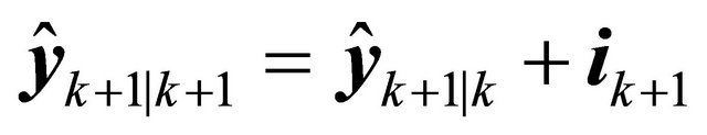 (6)
(6)
Here, the information contribution matrix and the information contribution vector are defined as follows, respectively [4,5]:
 (7)
(7)
 (8)
(8)
Information Fusion
In the sensor fusion literature, there are a number of sensor networks with their own virtues and limitations [2]. In this paper, we specifically consider a distributed configuration with feedback [3]. As shown in Figure 1, in this network, each local sensor has its own information processor. The locally processed results are then transmitted to the fusion center for computing a global estimate. The global estimate is broadcast so that all the local sensors utilize the global estimate for the purpose of processing the next measurement. The advantage of using the information filters within the local sensors is that the global estimate in the fusion center can be computed from  sensor measurements at each time step by simply summing the local information vectors and matrices:
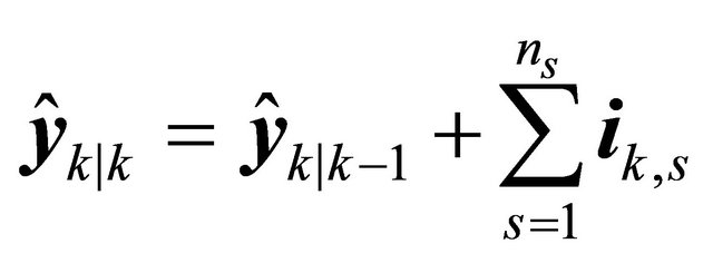 (9)
(9)
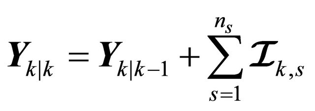 (10)
(10)
Note that the computations outlined in this section hold under the following assumptions: 1) The tracking problem at hand is described by a linear Gaussian system; 2) The sensor measurements are uncorrelated to each other; 3) There is no measurement origin of ambiguity; 4) The sensors are synchronized; 5) There is no receipt of out-of sequence measurements; 6) There is no communication loss among sensors. When one or more of these conditions are violated, various techniques have been proposed to get around them in the literature [2].
3. Square-Root Cubature Information Filtering
In each recursion cycle, it is important that we preserve the two properties of an information matrix, namely, its positive definitiveness and symmetry. Unfortunately, when the CIF is committed to an embedded system with limited word-length, numerical errors may lead to a loss of these properties. The accumulation of numerical errors may cause the information filter to diverge or otherwise crash. The CIF involves numerically sensitive operations such as matrix square-rooting and matrix inversion, which may combine to destroy the fundamental properties of an information matrix. The logical procedure to preserve both properties of the information matrix and to improve the numerical stability is to design a square-root version of the CIF. Although the square-root cubature information filter (SCIF) is reformulated to propagate the square-roots of the information matrices, both the CIF and the SCIF are algebraically equivalent to other.
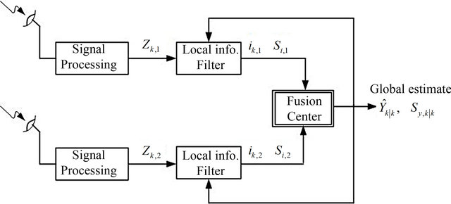
Figure 1. Information flow in a distributed sensor configuration with feedback.
Before deriving the SCIF, for convenience, we introduce the following notations:
• We denote a general triangularization algorithm (e.g., QR decompositio n) as , where
  is a lower triangular matrix. The matrices
  and
and  are related to each other as follows: Let
  be an upper triangular matrix obtained from the QR decomposition on
 ; then
 .
.
• We use ![]() and
and ![]() to denote the square-roots of
to denote the square-roots of  and
and , respectively. That is,
  and
and .
.
Because many of the SCIF computations can be easily borrowed from the SCKF [7], we only derive the steps that require explicit treatments in the sequel. Like the SCKF, the SCIF also includes two steps, namely, the time update and the measurement update.
3.1. Time Update
Let  be
be
 (11)
(11)
and  be
be
 (12)
(12)
As depicted in Figure 2, the time update of the SCIF connects  to
to  via three paths. Let us first consider how to derive Path 1, in which the information space is projected onto the state space. Taking inverse on both sides of (1), we get
 (13)
(13)
Substituting the square-root factors on both side of (13) yields
 (14)
(14)
We may therefore write the square-root of the error covariance matrix
 (15)
(15)
We summarize the following important result from (13) and (15) as follows:
![]() (16)
(16)
Because  is a triangular matrix, the least-squares method can be used to avoid computing its inversion explicitly [8]. From (2), we write the updated state estimate
 (17)
(17)
which completes Path 1.
As shown in Figure 2, Path 3 is an inverse projection (from the state space to the information space) of Path 1. By closely following this idea and using (3), (4), the state space quantities can be projected back onto the information space to obtain Path 3. Because Path 2 is identical to the time update of the SCKF, the reader may refer to Section VII of [7] for a detailed derivation.
3.2. Measurement Update
In the measurement update step, we will see how to fuse a new measurement with the predicted information to obtain the updated information. As depicted in Figure 3, the measurement update step also includes three paths. Consider Path 1. Given  and
and , the predicted measurement
  and the sub-matrices of the transformation matrix
 , namely,
  and
and  can be obtained as described in Section VII of [7]. Fortunately,
  and
and  are available as the by-products of the time update of the SCIF, specifically, from Path 2 of the time update. For this reason, we do not describe the derivation of Path 1 in this paper.
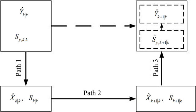
Figure 2. Time update of the SCIF.
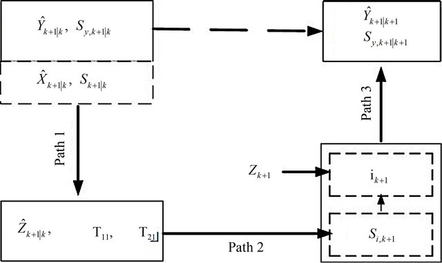
Figure 3. Measurement update of the SCIF.
Let us derive Path 2 now. The end products of Path 2 are the information contribution vector , and the square-root information contribution matrix
 . First, we will derive
 . By closely following (16), we may write the inverse of the measurement noise covariance matrix
 (18)
(18)
Substituting (18) into (7) and rearranging the right hand side, we get
 (19)
(19)
Therefore, from (19), we may write  in a factored form:
 (20)
(20)
where the square-root information matrix of dimension  is defined as
 (21)
(21)
 (22)
(22)
Because  (see Equation (37) of [7]), we finally write (22) as
![]() (23)
(23)
To determining , we rewrite (4) as
 (24)
(24)
Because  is a symmetric matrix, we may also write (24) as
 (25)
(25)
Substituting (25) into (8) yields
 (26)
(26)
Substituting (21) into (26) and expanding the right hand side yields
 (27)
(27)
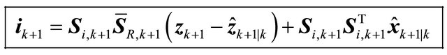
Consider Path 3 now. The updated information vector  can be computed by substituting (27) into (6). To obtain the updated information matrix
 , we replace the right hand side of with square-roots and write
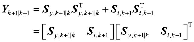
Hence, the square-root of the updated information matrix is given by
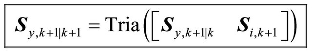 (28)
(28)
Note: When the local sensors employ the square-root information filtering algorithm, they are required to send the square-root information matrices to the fusion center (see Figure 1). For a distributed sensor network with  sensors, we may obtain
  by augmenting the arguments on the right hand side of (28) with
  squareroot information contribution matrices coming from
  sensors.
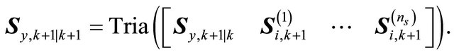 (29)
(29)
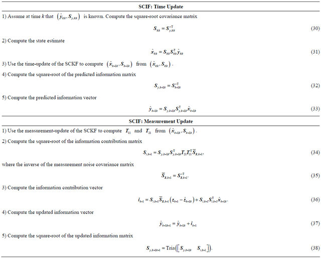
Table 1 below summarizes the steps involved in the SCIF algorithm.
Table 1. SCIF algorithm
4. Application to Decentralized Sensor Fusion
Context. We consider an air-traffic control scenario, where an aircraft executes maneuvering turn in a horizontal plane at a constant, but unknown turn rate . Figure 4 shows a representative trajectory of the aircraft. The kinematics of the turning motion can be modeled by the following nonlinear process equation [1]:
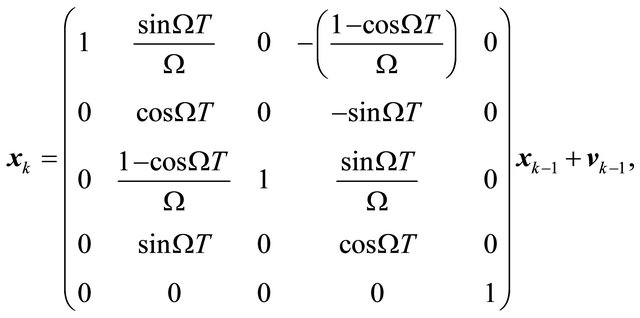
where the state of the aircraft
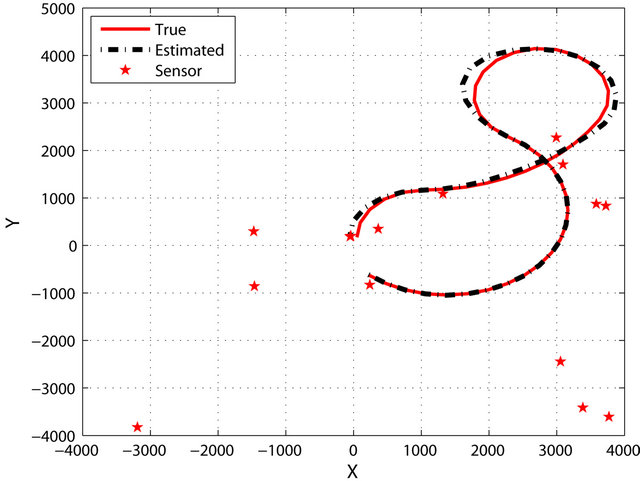
Figure 4. True aircraft trajectory—solid line, SCIF estimate—dotted line,![]() —Radar locations.
—Radar locations.
 ;
;  and
and  denote positions, and
  and
and  denote velocities in the x and y directions, respectively; T is the time-interval between two consecutive measurements; the process noise
  with a nonsingular covariance
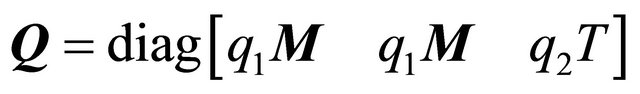 , where
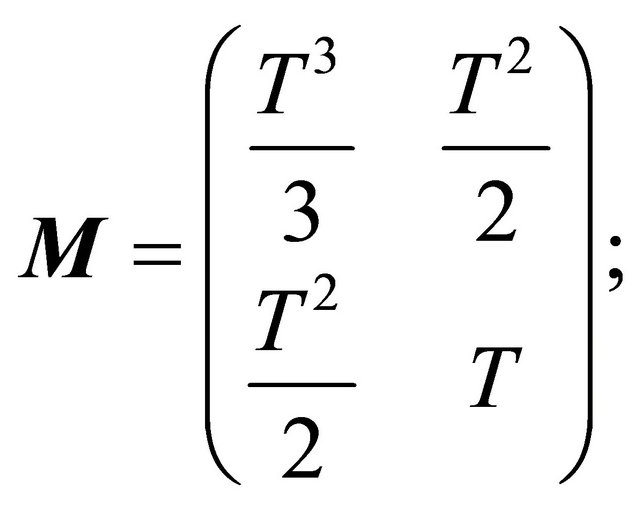
The scalar parameters  and
and  are related to process noise intensities. The radars were assumed to measure range and range-rate. For a radar located at
  , the measurement equation is given by
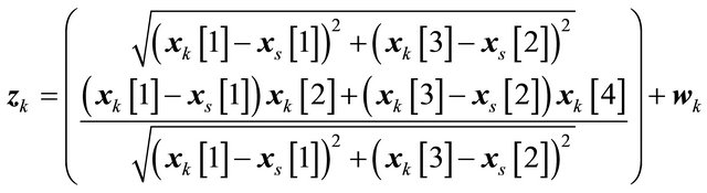 (39)
(39)
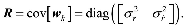
where the measurement noise covariance  is given by
To make this nonlinear tracking problem highly difficult, the target trajectory was made up of four segments, in each of which  was set to be
  and
and  for the duration of 0 - 40 s, 40 - 70 s, 70 - 90 s and 90 - 100 s, respectively. We used the following parameters for simulation:


The true initial state was assumed to be at

The initial state estimate  was chosen randomly from
  in each run, where

For a fair evaluation, we made a total of  independent Monte Carlo runs (The reader may refer to https://sites.google.com/site/haranarasaratnam/software for a set of Matlab code used to generate the results). The radars were randomly placed in a square-shaped surveillance region with the opposite vertices at (–4000, –4000) and (4000, 4000). In this experiment, the number of radars,
  , was varied from one to fifteen. We employed the following information filters for tracking the aircraft:
• Extended Information Filter (EIF);
• Cubature Information Filter (CIF);
• Square-root Cubature Information Filter (SCIF).
Note that the unscented information filter boils down to the CIF when the free parameter ![]() is forced to take zero. For this reason, the unscented information filter was excluded from comparison.
is forced to take zero. For this reason, the unscented information filter was excluded from comparison.
Performance Metrics. For performance comparison, we computed the accumulative root mean-squared error (ARMSE) in position and velocity. The ARMSE yields a combined measure of the bias and variance of a filter estimate. We define the ARMSE in position

where  and
and  are the true and globally estimated positions at the n-th Monte Carlo run. Similarly to the ARMSE in position, we may also write formula of the ARMSE in velocity. To check the numerical robustness of an information filter, the filter divergence rate was introduced. The filter was declared to diverge when
 ![]() of a specific Monte Carlo run exceeded 100 m. Subsequently, those diverged runs were excluded from the final calculations of
of a specific Monte Carlo run exceeded 100 m. Subsequently, those diverged runs were excluded from the final calculations of  and
and .
.
Observations. Figures 5(a) and (b) show the ARMSE in position and velocity, respectively, for the SCIF and EIF. As expected, as the number of sensors  increases, the ARMSEs in position and velocity decrease. However, the performance gain quickly diminishes; as
 , the performance gain seems to be trivial. Moreover, the SCIF consistently outperforms the EIF irrespective of
  although the performance deviation between the two reduces with
 . The CIF is not included in Figures 5(a) and (b) because its performance was almost identical to the SCIF.
Figure 6 shows how many times each filter experienced divergence out of N = 100 independent Monte Carlo runs. As can be seen from Figure 6, the EIF diverges the most. However, its divergence rate decreases as ns increases. The CIF diverges a few times especially when ns is less. The SCIF diverges a few times only when ns = 2. Unlike the CIF, the SCIF does not diverge when ns = 3 and 4. This observation indicates that the SCIF is superior to other filters in terms of numerical robustness. None of the filters diverged when .
.
5. Concluding Remarks
This paper has presented a numerically robust square-root

(a) Position Error (m)

(b) Velocity Error (m/s)
Figure 5. Accumulative root mean-squared error.
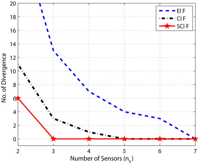
Figure 6. Number of divergence experienced in 100 independent Monte Carlo runs.
cubature information filter (SCIF) algorithm for multisensor fusion in a nonlinear Gaussian environment. Because the SCIF propagates the square-root matrices, it avoids to compute numerically sensitive matrix calculations. It was successfully demonstrated that the proposed SCIF algorithm is numerically robust using a computer experiment in which a target tracking problem in a distributed sensor network with feedback was considered. One of the interesting future research topics is to compare the computational demands of various information filters.
REFERENCES
- Y. Bar Shalom, X. R. Li and T. Kirubarajan, “Estimation with Applications to Tracking and Navigation,” Wiley & Sons, New York, 2001. doi:10.1002/0471221279
- Y. Bar-Shalom and X. R. Li, “Multitarget-Multisensor Tracking: Principles and Techniques,” YBS, Storrs, 1995.
- Y. Zhu, Z. You, J. Zhao, K. Zhang and X. Li, “The Optimality for the Distributed Kalman Filtering Fusion,” Automatica, Vol. 37, No. 9, 2001, pp. 1489-1493. doi:10.1016/S0005-1098(01)00074-7
- T. Vercauteren and X. Wang, “Decentralized Sigma-Point Information Filters for Target Tracking in Collaborative Sensor Networks,” IEEE Transactions on Signal Processing, Vol. 53, No. 8, 2005, pp. 2997-3009. doi:10.1109/TSP.2005.851106
- Y. Kim, J. Lee, H. Do, B. Kim, T. Tanikawa, K. Ohba, G. Lee and J. Yun, “Unscented Information Filtering Method for Reducing Multiple Sensor Registration Error,” IEEE International Conference on Multisensor Fusion and Integration for Intelligent Systems, Seoul, 20-22 August 2008, pp. 326-331. doi:10.1109/MFI.2008.4648086
- I. Arasaratnam and S. Haykin, “Cubature Kalman Filters,” IEEE Transactions on Automatic Control, Vol. 54, No. 6, 2009, pp. 1254-1269.
- I. Arasaratnam, S. Haykin and T. R. Hurd, “Cubature Kalman Filtering for Continuous-Discrete Systems: Theory and Simulations,” IEEE Transactions on Signal Processing, Vol. 58, No. 10, 2010, pp. 4977-4993.
- G. H. Golub and C. F. Van Loan, “Matrix Computations,” MD John Hopkins University Press, Baltimore, 1996.