Materials Sciences and Applications
Vol.08 No.11(2017), Article ID:79576,17 pages
10.4236/msa.2017.811055
Prediction of Weld Joint Shape and Dimensions in Laser Welding Using a 3D Modeling and Experimental Validation
Laurent Jacques, Abderrazak El Ouafi
Engineering Department, University of Quebec at Rimouski, Rimouski, Canada

Copyright © 2017 by authors and Scientific Research Publishing Inc.
This work is licensed under the Creative Commons Attribution International License (CC BY 4.0).
http://creativecommons.org/licenses/by/4.0/


Received: July 26, 2017; Accepted: October 9, 2017; Published: October 12, 2017
ABSTRACT
This paper presents an experimentally validated weld joint shape and dimensions predictive 3D modeling for low carbon galvanized steel in butt-joint configurations. The proposed modelling approach is based on metallurgical transformations using temperature dependent material properties and the enthalpy method. Conduction and keyhole modes welding are investigated using surface and volumetric heat sources, respectively. Transition between the heat sources is carried out according to the power density and interaction time. Simulations are carried out using 3D finite element model on commercial software. The simulation results of the weld shape and dimensions are validated using a structured experimental investigation based on Taguchi method. Experimental validation conducted on a 3 kW Nd: YAG laser source reveals that the modelling approach can provide not only a consistent and accurate prediction of the weld characteristics under variable welding parameters and conditions but also a comprehensive and quantitative analysis of process parameters effects. The results show great concordance between predicted and measured values for the weld joint shape and dimensions.
Keywords:
Laser Welding, Finite Element Method, 3D Modeling, Numerical Simulation, Weld Shape, Weld Dimensions, Predictive Modeling

1. Introduction
The laser welding process has gained importance in fabrication industries due to its ability to produce precise welds with small heat affected zones [1] . It is a complex process using thermodynamic, fluid flow, phase transition and heat transfer phenomena. Since laser welding experiments are rather long and expensive, finite element simulations are widely used to predict optimal parameters in various industrial applications. Simulation efforts can also be used to understand the process by facilitating the investigation inside the welding zone. Because of the welding process simulation is difficult to be completed using only one model, two types of models are considered. The multi-physic based model is used to acquire reliable and accurate predictions of the thermal field and the weld shape. The thermo-mechanical based model is used to evaluate the mechanical stress and strain due to the welding process.
Conduction mode and keyhole mode are the two basic modes for laser welding. Conduction mode is defined by low energy concentration and shallow penetration. Keyhole mode is defined by high energy concentration and deep penetration achieved when the metal vaporizes and forms a deep and narrow vapour cavity. However, there is no sharp transition between the two modes; a transition zone exists and can be defined by a constant aspect ratio. It has been found that the value of the transition zone ratio varies with laser beam diameter and speed [2] . For a model to be able to simulate both modes, the formation of the keyhole has to be simulated, or different heat sources have to be used for conduction and keyhole mode [3] . In this study two heat sources are used. One for the conduction mode and the other for the transition and the keyhole modes.
The multi-physical aspect of the laser process is the main difficulty in their modelling, as phenomena are coupled and different scales of physics interact [4] . Laser welding models are becoming very sophisticated using a free surface tracking method. A brief literature review of laser welding simulation is outlined here, and more details can be found in the review produced by Mackwood [5] . The first attempts to simulate laser welding were mostly based on Rosenthal’s [6] analytical solution of heat conduction equations with a point heat source moving on the surface of a semi-infinite plate. Then Eagar and Tsai [7] improved Rosenthal’s solution using a 2D Gaussian heat source. Later, Goldak was the first to come with a 3D heat source (double ellipsoidal) in finite element simulation, which was well adapted for high penetration laser welding [8] . The most recent simulations for scientific purposes have fluid flow, simulate plasma and vapour, and give precise predictions of the temperature inside the keyhole and its shape [9] [10] [11] . Models used to predict optimal parameters are simpler using methods to minimize the number of parameter and the calculation time. Those kinds of models use different heat source distributions, parameters and methods to account for different phenomena. A 3D finite element simulation with a high density heat source has been performed with ANSYS to predict the temperature field [12] . The heat source is a combination of a 3D conical Gaussian heat source and a surface Gaussian heat source, with the surface heat source representing 25% of the power absorbed and the volumetric heat source 75%. Another study has been conducted looking at the effect of the fluid flow on the melt pool shape [13] . The study investigates the nonlinear material properties and the effects of three laser heat sources.
In butt joint laser welding, the presence of a gap between sheets has an impact on the weld pool. However, gap is hard to add to a simulation without making it very complex. A study has been conducted on the deformation caused by thermally induced stresses that can result in a change of the gap width between the welded parts [14] . These displacements are studied through both experiments and simulations. The numerical simulation only represents the displacements; no gap bridging is done in the simulation. An investigation on gap bridging of pulsed laser welding reveals an advanced finite element model with fluid motion and free surface physics [15] . The effect of many parameters on the ability of gap bridging is examined. The 2D finite element model is able to model the joining of a butt joint and overlap joint with gap. However, no experimental validations have been done on the weld dimensions and underfill.
This paper presents a simple heat transfer model based on a moving heat source on a finite medium. The weld pool shape and dimensions are studied in continuous wave butt joint laser welding. The particularity of this simulation is the addition of the gap as a parameter of the simulation, and the prediction of the underfill for a full penetration weld. Conduction mode and keyhole mode are also covered in this model, using different heat sources according to the power density and interaction time. A 3 kW Nd: YAG laser for welding low carbon galvanized steel is used for the experimental investigation.
2. Heat Transfer Formulation
Heat transfer is the main phenomenon explaining the thermal field in laser welding. The fundamental modes of heat transfer are conduction, convection and radiation. Conduction occurs inside the parts. Convection and radiation occur between the parts and its environment.
2.1. Heat Transfer Equation
The law of heat conduction states that the time rate of heat transfer through a material is proportional to the negative gradient in temperature and to the area. As an equation, it can be written as:
(1)
where k is the thermal conductivity, the temperature gradient and φ the heat flux.
According to the law of conservation of energy, the internal heat transfer equation is:
(2)
where ρ is the mass density, Cp the specific heat and a distributed volume heat source.
2.2. Boundary and Initial Conditions
In order to solve the differential equations, initial conditions and boundary conditions must be specified. Initial conditions are the ambient temperature and parts temperature. Both are fixed at a temperature T0 equal to 20˚C. Boundary conditions are prescribed, thermal flux coming from radiation and convection. Convection is the thermal exchange resulting from the temperature difference between a body and its environment. The convective heat transfer can be defined by:
(3)
where h defined asthe convective heat transfer coefficient and T0 the room temperature.
The convective heat transfer coefficient highly depends on the fluid flow around the parts. Since ventilation is used during welding, a forced convection coefficient is used. Radiation occurs in the form of electromagnetic waves. According to the Stefan-Boltzmann law, when a hot object is radiating energy to its cooler surroundings, the radiation heat loss can be expressed as:
(4)
where σ is the Stefan-Boltzmann constant and ε the emissivity. These boundary conditions are applied to the model by specifying the value of the heat flux at the outward boundary of the model. The heat transfer modes through the parts are represented in Figure 1.
2.3. Heat Source Model
The heat source distribution is an influential parameter in laser welding models. Two kinds of heat source models exist for simulating laser welding: surface heat source and volumetric heat source. The surface heat source model is more accurate for conduction welding since in this mode the energy is applied to the component surface, while the volumetric heat source is more adapted for keyhole welding, with the energy being directed inside the medium through the keyhole [3] . The volumetric heat sources are the most studied distribution for

Figure 1. Heat transfer condition.
the simulation of laser welding, and many different kinds have been developed over the years [16] . Recent volumetric heat source models are combinations of double ellipsoidal, cylindrical, and conical models [17] . A simple efficient model is a 3D conical Gaussian heat source [18] . It is defined by a 2D Gaussian distribution for every height. Figure 2 represents a 3D conical Gaussian heat source. It can be seen that the power density is maximum at the top surface and decreases through the penetration zone. The energy is distributed throughout the thickness. The most of the energy is absorbed at the top surface, then the received energy decreases with the dimension of the keyhole. That is why volumetric heat sources are necessary to model keyhole mode laser welding. The 3D conical Gaussian heat source can be written as:
(5)
where Q0 is the power, Rc the reflection coefficient, Ac the absorption coefficient, σx and σy the radius of the heat source along x and y.
Complex models exist for the conduction mode, such as an adaptive volumetric heat source [19] . Buta 2D Gaussian heat source is a decent compromise between accuracy and simplicity. It is defined by:
(6)
3. Model Description
The model is based on a moving heat source over a steel plate. The heat transfer equations are used to determine the thermal field using the finite element method. In building the model, the following assumptions were considered: 1) The surfaces of the parts are assumed to be flat permitting perfect contacts; 2) the areas with temperatures higher than liquidus are considered molten; 3) the

Figure 2. 3D conical Gaussian distribution [20] .
vaporisation of elements is not simulated and laser interaction with vapour plumes is not studied; 4) the fluid dynamics are not considered; and 5) The temperature field is supposed to be symmetrical in the welding line.
3.1. Symmetry Simplification
Since there is geometrical symmetry along the weld line, only one sheet can be modelled using a symmetry boundary condition if the thermal field is also symmetrical. Three stages are present during the laser heating process: a starting stage at which the initiation of the weld begins with the heat source reaching the parts; a quasi-stationary stage at which the heat source is moving along a straight line and the temperature distribution is stationary; and finally an ending stage when the heat source leaves the parts [20] . Since the heat source is symmetrical and both sheets are supposed to be identical with perfect contact between them, it is assumed that the temperature field reached in the quasi-stationary state has symmetry along the weld direction line. Even though the temperature field might not be symmetrical during the initial and final stages, the assumption is made that the use of symmetry does not change the quasi-stationary stage reached. This assumption neglects misalignment of the laser and contact inaccuracy between sheets.
3.2. Phase Transition
During phase transitions, energy is absorbed or released by the body proportionally to its latent heat, with material properties varying according to the new phase. Different methods can be used to develop a finite element model of laser welding that considers phase change [16] . The most accurate way that avoids multi-physical phenomena is to consider temperature-dependent thermo-physical material properties (density, specific heat, and thermal conductivity). With this method, variations of thermal properties due to phase transitions are considered, but the effect of latent heat is neglected. Since latent heat has a significant effect on the melt pool, methods have been created to account for it [21] . With the enthalpy method, the energy absorbed by latent heat is added to the specific heat with modifications calculated from the enthalpy [13] . The use of a non-multi-physical simulation drastically reduces the solving time, but ignores the fluid dynamics of the liquid and vapor phases.
3.3. Welding Mode
The main difference between conduction mode and keyhole mode is the power density applied to the welding area. The power density is determined by two laser parameters, laser beam diameter and power. Those parameters are inputs of the simulation. A transition mode exists between the two modes, during which the aspect ratio (depth to width ratio) stays nearly constant with increasing power density. The beginning of the transition mode is called the upper limit of conduction mode. The upper limit of conduction mode depends on the interaction time, which is the laser beam diameter divided by the speed [21] . Figure 3

Figure 3. Welding mode according to power density and interaction time.
represents the welding mode according to previous experimentation. The upper limit for conduction mode has been found to be 0.94 MW/cm2 power density for a 9 ms interaction time, and 1.26 MW/cm2 for a 3.4 ms interaction time. The limit is supposed to vary linearly with the interaction time. In the model the power density and interaction time are calculated and compared to this limit in order to choose the heat source to be used. The conduction heat source is selected below this limit, while the keyhole heat source is selected above it.
3.4. Gap Effects
A purpose of this simulation is to predict the dimensions of a weld with a gap. Since the melted metal (liquid phase) and the fluid flow are not simulated, a gap cannot simply be placed between the sheets in the model. According to a previous analysis of variance conducted through experimentation, gap effects increase the depth and reduce the width, which are opposite of the effects of diameter. Other parameters used in this study increase or decrease both the penetration and the width. To simulate the effect of the gap a multiplier coefficient G is added to the laser beam diameter in the heat source formula. A heat source with modified diameter can be written as:
(7)
Since the effect of the gap is the opposite of the diameter, the coefficient has to be less than 1. After some tests, a value of 0.75 has been found to be relevant, which represents a decrease of about 0.1mm in diameter.
3.5. Impact of the Underfill
In butt joint laser welding, the two main factors that create a lack of material in the weld are edge straightness and sheet positioning. The main factor that generates an excess of material is the stress created during cooling. For partial penetration welds, the underfill has no direct impact on the dimensions of the weld. The presence of an underfill simply moves the weld deeper into the parts. For full penetration welds the underfill reduces the depth of the weld, causing it to be less than the thickness. Since the underfill is not evaluated in this simulation, results will always indicate a depth of penetration equal to the thickness of the sheets. Therefore, another method is used to obtain the dimensions of the underfill in order to estimate the correct dimensions of the full penetration weld. It has been seen in a previous study that the underfill is linked to the thickness, the edge straightness, the gap, and the width of the weld for full penetration welds. Using this information, an estimation of the underfill can be made from those parameters. The empirical formula giving the underfill as a percentage of the thickness for a full penetration weld, inspired from the gap bridging formula [22] , can be written as:
(8)
where g is the gap size, t the thickness, E the edge preparation coefficient (5% is used here), and BDW the bead width. Simulated full penetration welds calculate the underfill using this formula. The underfill is then subtracted from the penetration in order to determine the effective penetration.
4. Finite Element Model
The laser welding simulation can be simplified as a sheet with a laser moving along its length, as represented in Figure 4. The finite element model is created with the “heat transfer in solid” module of COMSOL Multiphysics, a software for numerical simulation.
Tetrahedron elements are chosen for the mesh because of their fast, easy meshing and refining. In order to have an accurate temperature field in the region of high temperature gradients, a dense mesh is used close to the weld line, while in the more distant region a coarser mesh is used, as can be seen in Figure 5. The thinnest elements are found along the weld line, with a width under 20 µm to minimize temperature error and provide good precision. The simulation time is calculated according to the welding speed and the length of the specimen.

Figure 4. Schematic model for laser welding.

Figure 5. Finite element mesh of the weld specimen.
The time steps are chosen according to the welding speed and the diameter. So that for each new time step, the laser beam diameter covers 1/3 of the beam’s coverage during the previous time step.
Many parameters are required to simulate laser welding: materials and optic properties, laser parameters, and parts dimensions [23] . Experimentation used for modelling validation needs the selection of the parameters that have most influence. The used specimens are galvanized steel A635CS cut to 30 mm × 50 mm using hydraulic shear. The edge did not receive further treatment. Laser power, welding speed, sheet thickness, beam diameter and gap were the parameters used in this study. These factors were used to generate an experimental design of 54 tests.
4.1. Material Properties
Material properties have a strong influence on heat transfer. Some material properties are taken dependant of the temperature. During laser welding the temperature varies between 20˚C and over 5000˚C. Since there is no easy theoretical formula to interpolate properties over such a temperature range, experimental data is the main way to access to those values. But experimentation is expensive and difficult. The temperature dependant properties are often not available for a precise grade. The properties of another grade of steel can provide a good approximation. The used properties are supplied by Abhilash for 904L steel [24] , which is a low carbon stainless steel. Table 1 shows the temperature independent properties, which include standard metal properties and two optical properties. The optical properties depend on the material surface and the type of laser. In this study galvanized steel and an Nd: YAG laser are used [25] . The absorption coefficient represents the power density attenuation per length unit and the reflection coefficient represents the percentage of the reflected laser beam. Figure 6 shows the temperature effects on specific material thermo-physical properties. The increase in specific heat at liquid us temperature is caused by the enthalpy method used to model the heat absorbed by the latent heat of fusion.
 (a)
(a)
 (b)
(b)
 (c)
(c)
Figure 6. Thermo-physical properties of material-Temperature effects on: (a) Specific heat; (b) Density and (c) Thermal conductivity.

Table 1. Specifications of the used material.
4.2. Process Parameters
The process parameters such as power, diameter and speed are easily adjustable. The same process parameters are used for the simulation and for the validation. Each parameter have 3 levels, which can be seen in Table 2. For the sheet dimensions, three different thicknesses are used according to the experiment. Since measurements are taken in the quasi stationary state, length and width are chosen to reach this state minimizing the size of the solid. The dimensions selected are shown in Table 3.
Table 2. Welding process parameters.
Table 3. Dimensions of the used parts.
5. Results and Discussion
The values of bead width (BDW) and depth of penetration (DOP) of the weld are measured on the thermal fields using the concept that the limit of the melted pool is the liquidus temperature. Since modifications have been added to the simulation for gap, conduction mode, and full penetration weld, each condition is looked at individually.
5.1. Comparison of Predicted and Measured Weld Dimensions
5.1.1. Predicted and Measured Weld Dimensions with No Gap
The predicted and measured BDW and DOP values for tests without gap are presented in Table 4. The comparison of the measured and predicted DOP and BDW is graphically illustrated in Figure 7. The results reveal that the predicted DOP and BDW are in good agreement with the experimental observations with small average errors of 6% and 11% for DOP and BDW respectively.
5.1.2. Predicted and Measured Weld Dimensions with Gap
The predicted and measured BDW and DOP for the gap test are presented in Table 5. The graphs of predicted and measured DOP and BDW are represented in Figure 8. The results show an average error of 5% for DOP and 14% for BDW indicating that BDW is more difficult to model than DOP. The DOP prediction is excellent, while the BDW prediction of is slightly less accurate. The method used to model the gap appears effective with no difference in errors with and without gap. The additional error in BDW found for all the tests might therefore come from the keyhole heat source model.
5.1.3. Conduction Mode
Experiment numbers 4, 5, 6, 16, 17 and 18 are in conduction mode Table 4. Figure 9 shows predicted versus measured DOP and BDW for conduction mode trials. Slightly better results are found than for the keyhole tests, with an average

Figure 7. Predicted versus measured DOP and DOP (no gap test).
Table 4. Comparaison of measured andpredictedDOP and BDW(no gap test).
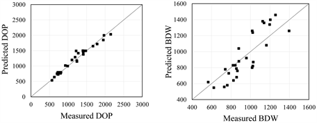
Figure 8. Predicted versus measured DOP and DOP (gap test).
Table 5. Comparaison of measured and predicted DOP and BDW (gap test).
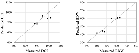
Figure 9. Predicted versus measured DOP and DOP (conduction mode).
error of 5% for DOP and 6% for BDW. The use of a conduction heat source turns out to be effective when doing low power density welds. A single heat source cannot be used to generate all the results within a high range of parameters.
5.1.4. Full Penetration Weld
Twenty simulations indicated full penetration, with depth equal to the thickness, as shown in Table 4 and Table 5. For those experiments, underfill has been evaluated and subtracted as explained. This change only impacts the depth. Since the width is used to evaluate the underfill, any error in width translates to error in depth. An average error of 6% for DOP is observed. Results are presented in Figure 10. This method produces good results for full penetration weld dimensions, for welds with and without gap. It also successfully takes into account the edge preparation to estimate the effective weld dimensions.
5.2. Macrograph of the Weld
Observation of the weld profile is used to evaluate if the general shape of the weld is in agreement with the experiment. In Figure 11, the pictures of the experimental welds are on the left, and pictures of the simulated welds are on the right (the weld pool is shown in red). The figure represents macrographs of three welds: 1) a weld without gap in keyhole mode, 2) a weld with gap in keyhole mode, and 3) a weld without gap in conduction mode. Those welds represent the three types of shapes obtained during experimentation. For each shape, the macrograph of the simulated weld is very similar to the one obtained from the experiment. The use of different heat sources enables the approximation of a wide range of weld pool shapes.
Figure 12 presents the shape of the simulated weld for full penetration weld in two configurations, with either the bottom or top edge of the simulated weld lined up with the experimental macrograph. The second configuration fits the shape better. This coincides with the assumption made for partial penetration welds that the underfill only moves the start of the weld deeper into the parts. Using this configuration, the fact that the underfill is not modelled only slightly impacts the weld pool shape.

Figure 10. Predicted versus measured DOP and DOP (full penetration).
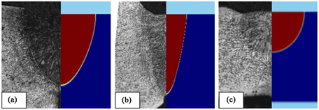
Figure 11. Shape of the bead profile from experimentation and simulation (a) Exp n˚3; (b) Exp n˚33; (c) Exp n˚16.

Figure 12. Shape of the bead profile from experimentation and simulation Exp n˚38 with (a) bottom edge lined up, (b) top edge lined up.
6. Conclusion
In this paper, an integrated approach used to build a weld joint shape and dimensions prediction model in laser welding for low carbon galvanized steel in butt-joint configurations is presented. Based on metallurgical transformations using temperature dependent material properties and the enthalpy method the modelling approach is used to investigate conduction and keyhole modes welding using surface and volumetric heat sources. A commercial 3 kW Nd: Yag laser system, a structured experimental design and confirmed statistical analysis tools are used to evaluate the modelling approach accuracy and to confirm the prediction model accuracy. Numerical simulation carried out through 3D FEM reveal great welds shapes and dimensions concordance between modelling and experimental results. The comparison of predicted and measured weld dimensions reveals similar accuracy for keyhole, conduction, full penetration and for gap welds. The prediction errors may have as sources the experimental errors as well as the adopted assumptions in the formulation, particularly for the fluid flow in the melt pool. The BDW presents a larger relative prediction error than DOP, probably because of the underfill (deeper experimental than simulation measurements). Globally, the results demonstrate that the numerical simulation can effectively lead to a consistent and accurate model and provide an appropriate prediction of the weld joint shape and dimensions under variable welding parameters and conditions.
Cite this paper
Jacques, L. and El Ouafi, A. (2017) Prediction of Weld Joint Shape and Dimensions in Laser Welding Using a 3D Modeling and Experimental Validation. Materials Sciences and Applications, 8, 757-773. https://doi.org/10.4236/msa.2017.811055
References
- 1. Mazumder, J. (1982) Laser Welding: State of the Art Review. Journal of the Minerals, metals, and Materials Society, 34, 16-24. https://doi.org/10.1007/BF03338045
- 2. Assuncao, E., Williams, S. and Yapp, D. (2012) Interaction Time and Beam Diameter Effects on the Conduction Mode Limit. Optics and Lasers in Engineering, 50, 823-828.
- 3. Kuang, J.H., Hung, T.P. and Chen, C.K. (2012) A Keyhole Volumetric Model for Weld Pool Analysis in Nd: YAG Pulsed Laser Welding. Optics & Laser Technology, 44, 1521-1528.
- 4. Otto, A. and Schmidt, M. (2010) Towards a Universal Numerical Simulation Model for Laser Material Processing. Physics Procedia, 5, 35-46.
- 5. Mackwood, A.P. and Crafer, R.C. (2005) Thermal Modelling of Laser Welding and Related Processes: A Literature Review. Optics & Laser Technology, 37, 99-115.
- 6. Rosenthal, D. (1946) The Theory of Moving Sources of Heat and Its Application to Metal Treatments. ASME, Cambridge.
- 7. Eagar, T. and Tsai, N. (1983) Temperature Fields Produced by Traveling Distributed Heat Sources. Welding Journal, 62, 346-355.
- 8. Goldak, J., Chakravarti, A. and Bibby, M. (1984) A New Finite Element Model for Welding Heat Sources. Metallurgical Transactions B, 15, 299-305. https://doi.org/10.1007/BF02667333
- 9. Pang, S., Chen, X., Zhou, J., Shao, X. and Wang, C. (2015) 3D Transient Multiphase Model for Keyhole, Vapor Plume, and Weld Pool Dynamics in Laser Welding including the Ambient Pressure Effect. Optics and Lasers in Engineering, 74, 47-58.
- 10. Chongbunwatana, K. (2014) Simulation of Vapour Keyhole and Weld Pool Dynamics during Laser Beam Welding. Production Engineering, 8, 499-511. https://doi.org/10.1007/s11740-014-0555-x
- 11. Abderrazak, K., Bannour, S., Mhiri, H., Lepalec, G. and Autric, M. (2009) Numerical and Experimental Study of Molten Pool Formation during Continuous Laser Welding of AZ91 Magnesium Alloy. Computational Materials Science, 44, 858-866. https://doi.org/10.1016/j.commatsci.2008.06.002
- 12. Shanmugam, N.S., Buvanashekaran, G. and Sankaranarayanasamy, K. (2010) Experimental Investigation and Finite Element Simulation of Laser Beam Welding of AISI 304 Stainless Steel Sheet. Experimental Techniques, 34, 25-36. https://doi.org/10.1111/j.1747-1567.2009.00552.x
- 13. Koo, B.S. (2013) Simulation of Melt Penetration and Fluid Flow Behavior during Laser Welding. Ph.D. Thesis, Lehigh University, Ann Arbor.
- 14. Nagel, F., Simon, F., Kümmel, B., Bergmann, J.P. and Hildebrand, J. (2014) Optimization Strategies for Laser Welding High Alloy Steel Sheets. Physics Procedia, 56, 1242-1251. https://doi.org/10.1016/j.phpro.2014.08.040
- 15. Roach, R.A., Fuerschbach, P.W., Bernal, J.E. and Norris, J.T. (2006) Thin Plate Gap Bridging Study for Nd:YAG Pulsed Laser Lap Welds. No. SAND2005-5356, Sandia National Laboratories. https://doi.org/10.2172/875619
- 16. Dal, M. and Fabbro, R. (2016) An Overview of the State of Art in Laser Welding Simulation. Optics & Laser Technology, 78, 2-14. https://doi.org/10.1016/j.optlastec.2015.09.015
- 17. Rahman Chukkan, J., Vasudevan, M., Muthukumaran, S., Ravi Kumar, R. and Chandrasekhar, N. (2015) Simulation of Laser Butt Welding of AISI 316l Stainless Steel Sheet Using Various Heat Sources and Experimental Validation. Journal of Materials Processing Technology, 219, 48-59. https://doi.org/10.1016/j.jmatprotec.2014.12.008
- 18. Kannatey-Asibu, E. (2009) Principles of Laser Materials Processing. John Wiley & Sons Ltd., Hoboken. https://doi.org/10.1002/9780470459300
- 19. Bag, S., Trivedi, A. and De, A. (2009) Development of a Finite Element Based Heat Transfer Model for Conduction Mode Laser Spot Welding Process Using an Adaptive Volumetric Heat Source. International Journal of Thermal Sciences, 48, 1923-1931. https://doi.org/10.1016/j.ijthermalsci.2009.02.010
- 20. Shanmugam, N.S., Buvanashekaran, G., Sankaranarayanasamy, K. and Ramesh Kumar, S. (2010) A Transient Finite Element Simulation of the Temperature and Bead Profiles of T-Joint Laser Welds. Materials & Design, 31, 4528-4542. https://doi.org/10.1016/j.matdes.2010.03.057
- 21. Van Elsen, M., Baelmans, M., Mercelis, P. and Kruth, J.P. (2007) Solutions for Modelling Moving Heat Sources in a Semi-Infinite Medium and Applications to Laser Material Processing. International Journal of Heat and Mass Transfer, 50, 4872-4882. https://doi.org/10.1016/j.ijheatmasstransfer.2007.02.044
- 22. Ready, J.F. and Farson, D.F. (2001) LIA Handbook of Laser Materials Processing. Laser Institute of America, Orlando.
- 23. Guan, Y., Yuan, G., Sun, S. and Zhao, G. (2013) Process Simulation and Optimization of Laser Tube Bending. The International Journal of Advanced Manufacturing Technology, 65, 333-342. https://doi.org/10.1007/s00170-012-4172-6
- 24. Abhilash, A.P. and Sathiya, P. (2011) Finite Element Simulation of Laser Welding of 904L Super Austenitic Stainless Steel. Transactions of the Indian Institute of Metals, 64, 409-416. https://doi.org/10.1007/s12666-011-0093-6
- 25. Kim, J.D. (1990) Prediction of the Penetration Depth in Laser Beam Welding. KSME Journal, 4, 32-39. https://doi.org/10.1007/BF02953388