Abstract

A classical field theory of gravity and electromagnetism is developed. The starting point of the theory is the Maxwell equations which are directly tied to the Riemann-Christoffel curvature tensor. This is done through the derivatives of the Maxwell tensor which are equated to a vector field contracted with the curvature tensor, i.e.,. The electromagnetic portion of the theory is shown to be equivalent to the classical Maxwell equations with the addition of a hidden variable. Because the proposed equations describing electromagnetism and gravity differ from the classical Maxwell-Einstein equations, their ability to describe classical physics is shown for several situations by direct calculation. The inclusion of antimatter and its behavior in a gravitational field, and the possibility of particle-like solutions exhibiting quantized charge, mass and angular momentum are discussed.

Keywords: Classical Field Theory, Gravitation and Electromagnetism, General Relativity, Antimatter, Antimatter Gravity, Hidden Variable Theories, Riemann Geometry

1. Introduction

Since the introduction of General Relativity, numerous classical field theories have been proposed which attempt to explain electromagnetism and gravitation in a unified and geometric framework [1] [2] . Many of these previous theories have proceeded by modifying the standard Riemann geometry or by working in more than 4 dimensions [3] -[5] . Here a new and unconventional approach to this problem is developed that offers the possibility of describing particles with both quantized charge and mass using a continuous 4-dimensional field theory and without making any modifications to the standard Riemann geometry. Although the general character of the solutions of the field equations proposed here is similar to that of General Relativity, the motivation for the equations is quite different. The motivation of Einstein’s field equations generally starts with a gravitational weak field analysis, and then progresses with some judicious guess work to. Here, instead of starting with that weak field analysis, the algebraic properties of the Riemann-Christoffel tensor are exploited to relate the Maxwell tensor and its derivatives to the curvature tensor. This leads naturally to a set of field equations that reduces in their weak field limit to the classical Maxwell equations and provides an underlying geometric basis for electromagnetism. Following this approach, the electromagnetic and gravitational field sources are treated as dynamical variables which when considering particle-like solutions become quantized through the application of appropriate boundary conditions.

More specifically, a continuous field theory is proposed with dynamical variables represented by two 2^nd-order tensor fields, two vector fields, and two scalar fields. All of these fields are familiar to classical physics with the exception of the vector field, which is used to couple the derivatives of the Maxwell tensor to the Riemann-Christoffel curvature tensor. The following is a list of the theory’s dynamical variables (fields):

: metric tensor;

: Maxwell tensor;

: 4-velocity;

: no counterpart in classical physics, used in

: charge density;

: ponderable mass density.

The outline of the paper is as follows. After describing the equations of the theory, I show that they are consistent with the requirements of general covariance, i.e., there are four degrees of freedom in the solutions of the dynamical variables of the theory corresponding to the four degrees of freedom in the choice of coordinate system. I then go on to find an exact spherically-symmetric solution for all dynamical variables representing the electric and gravitational fields of a point charge, which is in agreement with the asymptotic forms of these fields predicted by the conventional Maxwell-Einstein theory. A route to finding particle-like solutions having quantized mass, charge and angular momentum is then described, although exact solutions are not found. A discussion of antimatter, how it is included in the theory, and its behavior in gravitational fields are then given. Next I demonstrate a solution representing an electromagnetic plane wave in the weak field limit of the theory. Finally, I discuss the correspondence of the theory to classical electromagnetism. Throughout, emphasis is on the agreement of the proposed theory with the accepted understanding of classical physics (here classical physics refers to Maxwell-Einstein Theory).

Geometric units are used along with a metric tensor having signature [+, +, +, ‒]. Spatial indices run from 1 to 3, with 4 of the time index. For the definitions of the Riemann-Christoffel curvature tensor and the Ricci tensor, the conventions used by Weinberg are followed [6] .¹

2. Theory

A covariant theory of gravity and electromagnetism is developed by connecting the covariant derivatives of the Maxwell tensor directly to the Riemann-curvature tensor via contraction with a continuous vector field,

(1)

The motivations for this equation are the algebraic properties of the Riemann-curvature tensor. First, the cyclicity of the curvature tensor, , with (1) immediately gives Maxwell’s source-free equations,

, (2)

or equivalently, , since is antisymmetric. Second, Maxwell’s source-containing equations are then introduced by contracting the μ and κ indices in (1) to obtain

(3)

and noting that this forces

(4)

since vanishes identically by the antisymmetry of. The conserved vector field is identified with the conserved electromagnetic current density

(5)

where the subscript c stands for charge and is added for clarification and is the ordinary 4-velocity satisfying the normalization

(6)

In (5), is interpreted as the charge density that would be measured by an observer in the locally inertial coordinate system co-moving with the charge. Together, (3) and (5) then lead directly to Maxwell’s sourcecontaining equations,

(7)

An expression for can be derived from (5) and (6) in two equivalent but slightly different forms,

(8)

which will both be useful when looking for specific solutions. To complete the theory, a conserved energymomentum tensor is added,

(9)

where is the ponderable mass density and so always nonnegative. Contracting (9) with gives, which leads directly to

(10)

identifying as a locally conserved quantity. Combining (9) and (10) then gives

(11)

the Lorentz Force Law. The particular form of the energy-momentum tensor in (9) was chosen to ensure (10) and (11) as consequences. As described in the next section, the theory is logically consistent from the stand point of general covariance without need to impose any conditions on the stress-energy tensor beyond it being divergence free and of the form given in (9).

3. Logical Consistency and Completeness of Theory

The logical consistency and completeness of the theory is manifest in 22 independent relations that are used to determine the 26 dynamical fields of the theory. The 4-degrees of freedom in the determination of the dynamical variables are a result of general covariance. The dynamical variables of the theory are given in Table1

The equations of the theory are given in Table2

But not all of the equations of the theory listed in Table 2 are independent. Dependent equations which are derived from the equations in Table 2 are listed in Table3

The 11 dependent equations listed in Table 3, when applied against the 33 equations of the theory listed in Table 2, give a total of 22 independent equations.

4. Integrability Conditions

The approach presented here for electromagnetism and gravity departs from the standard Maxwell-Einstein description in the mixed system of first order partial differential equations that are used to describe the Maxwell tensor (1). It is not obvious at this point that (1) allows any solutions to exist due to the integrability conditions

Total = 26.

Total = 33.

Total = 11.

that must be satisfied by such a system for a solution to exist [7] . Although there are several ways of stating what these integrability conditions are, perhaps the simplest is given by

(12)

which is arrived at using the commutation relations for covariant derivatives. Using (1) to substitute for in (12) gives

(13)

which can be interpreted as conditions that are automatically satisfied by any solution consisting of expressions for, and that satisfy (1). In addition to the integrability conditions represented by (13), subsequent integrability conditions can be derived by repeatedly taking the covariant derivative of (13) and substituting in the resulting equation for using (1). The question that now arises is this: are these integrability conditions so restrictive that perhaps no solutions exist to the proposed theory? If so, and no solutions exist, then the theory is not interesting. But as will be shown in the next section, formal solutions satisfying the theory and representing particle-like fields which are in agreement with the classical Maxwell-Einstein theory in their asymptotic limit do exist. Additionally, radiative solutions valid in the weak field limit of the theory and representing electromagnetic plane waves are shown to exist. The existence of these formal solutions provides one of the motivations for further investigation of the theory.

5. Spherically Symmetric Solution

In this section solutions having spherical symmetry are investigated. Under these conditions, it is demonstrated that the Reissner-Nordstrom metric with an appropriate choice for is a formal solution of the theory, i.e., all equations in Table 2 are satisfied. Although the presentation in this section is purely formal, it is included here for several reasons. First, if the theory could not describe the asymptotic electric and gravitational fields of a point charge it would be of no interest on physical grounds. Second, the presented theory requires the solution of a mixed system of first order partial differential equations, a system that may be so restrictive that no solutions exist, and so at least a mechanical outline of one methodology to demonstrate a solution is warranted.

Starting with the Reissner-Nordstrom metric [8] ,

(14)

and a guess for,

(15)

where is a yet to be determined constant, is determined from the second form of (8) to be

(16)

where the positive root has been arbitrarily chosen. I’ll come back to this point later, but for now note that only nonnegative charge density is allowed by the theory with this choice for the root of (8). Using (5), is then found to be

(17)

The next step is to satisfy (1) by solving for. Rather than tackling this head on and trying to find a solution to (1), I will solve the integrability Equations (13), which are linear in for. Solving (13) in this manner, it is found that all the integrability equations are satisfied for given by

(18)

Choosing then gives an electric field that agrees with the Coulomb field of a point charge to leading order in. It is straightforward to substitute (18) into (1) and verify that (1) is now satisfied. The last remaining equation of the theory, the conserved energy-momentum Equation (9), is satisfied for given by

. (19)

This demonstrates that the values for the field quantities given in this section are an exact solution to the theory’s equations.

6. Quantization

The last step in the solution above in which the conserved energy-momentum Equation (9) was solved for demonstrates that formal solutions to the theory do exist. Because is a dynamical field of the proposed theory an additional physical constraint can be imposed on by requiring that it be self-consistent with the mass of the particle being modeled. This self-consistent mass can be determined by the gravitational field far from the particle, i.e., for large r. This constraint can be formulated quite generally for the static-metric, particle-like solutions being considered here as the following boundary condition,

, (20)

where is the determinant of the spatial metric tensor given by [9] ,

. (21)

In (21) i and j vary over the spatial indices only, and in (20) the factor appears in the integrand because it is the locally measured mass density where is the mass density that would be measured in the locally inertial coordinate system that is co-moving with it. The same type of self-consistency argument used above for quantizing mass can also be applied to charge, leading to quantized charge solutions. For the spherical coordinate system being considered here, the appropriate boundary condition on charge is

. (22)

For the spherically symmetric solution investigated in the previous section, the LHS of both (20) and (22) diverge leaving no hope for satisfying these boundary conditions. The upshot of this observation is that while representing a solution that describes the gravitational and electrical fields of a point charge and formally satisfying the equations of the theory in Table 2, the Reissner-Nordstrom metric solution cannot represent a physically allowed particle-like solution. The possibility of finding solutions that satisfy both the equations of the theory in Table 2 and the quantized mass and charge boundary conditions (20) and (22) remains an open question at this point. The reason for the absolute value of in boundary condition (20) for mass but not in boundary condition (22) for charge is driven by the symmetries of the equations of the theory in Table 2, and will be discussed more fully in the next section. Finally, if one goes to more generalized metrics that include nonzero angular momentum about an axis (cylindrically symmetric solutions) and so the possibility of magnetic fields, the line of thought used above to quantize the mass and charge of the particle can also be used to quantize its angular momentum.

7. Antimatter

The distinction between matter and antimatter in the theory is carried by the 4-velocity and the value that it takes on in the locally inertial co-moving coordinate system. In this coordinate system matter will have and antimatter will have. The spherically symmetric solution just investigated provides an illustration of this. In that solution, the value of the constant c₁ was chosen to be q/m. If q/m > 0, then the 4^th component of in (17) is positive, corresponding to matter. If, on the other hand, q/m < 0, then the 4^th component of is negative, corresponding to antimatter. This is the analogue of the view today that a particle’s antiparticle is the particle moving backwards through time [10] . With these definitions for the 4-velocity of matter and antimatter, charged ponderable mass density can annihilate similarly charged ponderable antimass density and satisfy both the local conservation of charge (4) and ponderable mass (10). Because total massenergy is conserved (9), the annihilation of ponderable matter and antimatter must be accompanied by the generation of electromagnetic energy, the only other available energy channel in the theory.

The following discussion further illuminates the definitions of matter and antimatter proposed above. For definiteness in what follows I will require always, corresponding to choosing the positive root in the second form of (8). With this requirement of only nonnegative charge density allowed by the theory, it will be useful to develop a test particle formalism to illustrate how test particles with an apparently negative charge can be handled in a self-consistent way. To do this I introduce a parameter s that takes on the value +1 for matter test particles and −1 for antimatter test particles

(23)

Consistent with the above definitions for matter and antimatter, the transformation from a test particle’s proper time interval dτ to a coordinate time interval dt is given by

(24)

and so the 4-velocity of a test particle is related to the ordinary 3-space velocity by

(25)

where γ has the usual definition. Now consider a region with an externally defined electromagnetic field

(26)

and with no, or at least a very weak, gravitational field so that and. Starting with the Lorentz Force Law (11) we have

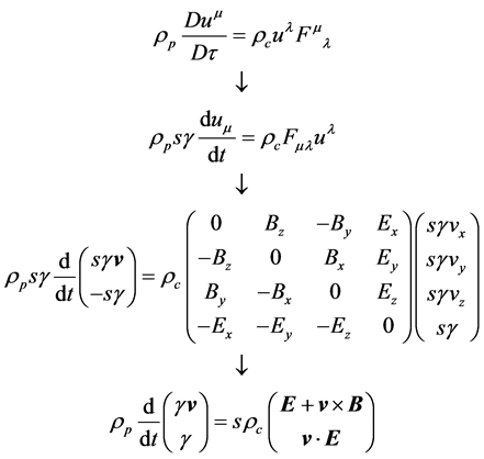(27)

which on the last line above ends up at the conventional form of the Lorentz Force Law except for the extra factor of s on the RHS. This extra factor of s in (27) gives the product s^.ρ_c the appearance of a negative charge density for antimatter and a positive charge density for matter.

The equations of the theory in Table 2 exhibit C-symmetry (charge conjugation symmetry), as for any matter solution there exists a corresponding antimatter solution via the field transformation

(28)

which leaves all equations in Table 2 unchanged. Using the already investigated Reissner-Nordstrom metric solution and the C-symmetry exhibited by the equations of the theory under transformation (28) one can now make predictions about the behavior of antimatter in an external gravitational field—is it attracted or repelled? As noted above in the investigation of the Reissner-Nordstrom metric solution, the difference between matter and antimatter solutions is dictated by the choice of sign of the charge-to-mass ratio q/m. Examining the ReissnerNordstrom metric (14) and noting that q appears always raised to the second power while m appears always to the first power (also true for the Kerr-Newman metric), the only way to ensure that matter solutions will have corresponding antimatter solutions with the same metrical structure is to require that the transformation from matter to corresponding antimatter solutions (changing the sign of the charge-to-mass ratio) be accomplished via the metric transformation and. This observation is the reason that the absolute value of is taken in the boundary condition (20) for mass but not in the boundary condition (22) for charge, and further motivates the requirement that ρ_p be always nonnegative. To answer the question of whether antimatter is attracted or repelled by a gravitational field, I go again to the Lorentz Force Law (11), but this time assume there is no electromagnetic field present at the location of the test particle, just a gravitational field corresponding to a Schwarzschild metric generated by a central mass m corresponding to either matter or antimatter, that is a distance r from the test particle, also matter or antimatter, which I take to be initially at rest. In this case the equation of motion of the test particle reduces to a geodesic trajectory as expected

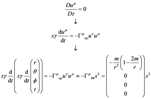(29)

where in the last line above I have approximated the RHS using the initial at rest value of and I have used the fact that the only nonzero in a Schwarzchild metric is. Further simplifying the first component of the last line in (29) by noting that initially, gives

(30)

independent of s, and so demonstrating that the proposed theory predicts that both matter and antimatter test particles will be attracted by a gravitational field generated by either matter or antimatter. The prediction of (30) that the gravitational interaction between matter and antimatter is mutually attractive is in contradiction to recent predictions based on the classical general relativity equations and their assumed CPT invariance [11] . There has recently been much interest in this issue due to possible explanations of dark matter [12] and dark energy density [13] . The planned AEgIS experiments (Antimatter Experiment: gravity, Interferometer, Spectroscopy) at CERN to measure the gravitational interaction between matter and antimatter may soon provide an experimental determination of this issue [14] .

8. Electromagnetic Plane Wave

In this section I investigate approximate solutions that represent electromagnetic plane waves. Throughout I work in the weak field limit with

(31)

where and, and I only retain the terms to 1^st order in the h’s. The coordinate system used is, and I assume a plane wave polarized in the x-direction and propagating in the +z-direction. This situation is described by the following Maxwell tensor,

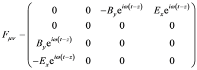(32)

To begin, I guess at a form for,

(33)

where c₁, c₂, c₃ and c₄ are yet to be determined constants. Next I impose (4), , which gives

(34)

There are two ways to solve (34), either or, but in the end it will not matter which is chosen, as both conditions will be required. Now imposing (1), we arrive at a series of constraints on the h’s and c’s that must be satisfied to the 1^st order in h. Rather than reproduce all of these equations here, I just give the results below, which are straightforward to verify by direct substitution.

(35)

In summary, the following metric tensor

(36)

with given by

(37)

describes an electromagnetic plane wave polarized in the x-direction and propagating in the +z-direction with electric field amplitude E_x. At this point the values of h₁₄, h₂₄, h₃₃, and c₄ in (36) and (37) are not restricted beyond the small field approximation for the h’s. The solution has the interesting property that the value of h₁₁ is only required to be nonzero to yield a physical solution for, but beyond that is unrestricted except for the weak field approximation if no further conditions are placed on.

9. Discussion

Taking a starting point that is distinctly different from that of the Maxwell-Einstein equations, the theory proposed here has been shown to agree with the predictions of the Maxwell-Einstein equations in the classical physics regime:

Ÿ  Equations (2) and (7) of the theory, are in the weak field limit exactly those of classical electromagnetism on Minkowski spacetime and so in the weak field limit the proposed theory corresponds to the classical Maxwell theory as already demonstrated for several physical situations. However, the proposed theory does not correspond exactly to classical electromagnetism because the Maxwell tensor is directly tied to the metric tensor and vice versa through (1). This is substantially different than the case in classical Maxwell-Einstein theory where the electromagnetic fields are at most coupled to the metric tensor through the energy-momentum tensor in Einstein’s General Relativity. An interesting observation is that if one only assumes knowledge of Equations (2) and (7) but not (1), as in classical electromagnetism, then the view from the perspective of the theory proposed here is that the classical description is incomplete, i.e., Maxwell’s equations are incomplete due to the hidden variable in (1), having no direct correspondence in classical physics.

Ÿ  Solutions representing the fields of point charges are shown to be described by the theory with electric fields in agreement to leading order in 1/r with those calculated using Maxwell’s equations, and their gravitational fields in agreement with those calculated using the Reissner-Nordstrom metric and General Relativity.

Ÿ  Electromagnetic plane waves are shown to be allowed weak field solutions of the theory, and because Maxwell’s equations are contained in the theory, the interaction of charged matter with electromagnetic fields is also described by the theory.

Ÿ  Although not presented in this manuscript, by following the same procedure as outlined for the ReissnerNordstrom metric in Section 5, one can show that the Kerr-Newman metric satisfies the equations of the theory to leading order in 1/r, demonstrating that the theory also allows the asymptotic field descriptions of a point charge superimposed on a magnetic dipole to leading order in 1/r.

It is in the sense that the above points encompass classical physics that it can be argued the theory correctly describes classical physics. However, the theory differs from the classical physics description in that the source terms of both gravitational fields and electromagnetic fields are deterministically described as dynamic variables (fields) by the theory. The theory as presented obeys the rigid requirements of being logically complete in that the all of the theory’s dynamic variables (fields) are given up to the requirements imposed by general covariance. This internal logic is manifest with the introduction of the vector field that has no counterpart in classical physics, but which is a well hidden variable in most circumstances. Specifically is hidden in the classical physics regime considered above by the identification of it with the charge current density given in (5), i.e., with that identification the theory yields the standard Maxwell equations. The fact that is so well hidden in what is a fully deterministic theory that replicates our understanding of physics in the classical regime, and the fact that is intimately tied to the charge density of particle-like solutions (5) makes it enticing to consider it as a bridge to quantum mechanical considerations.

A remarkable feature of the theory is that the gravitational field of particles is in agreement with that of General Relativity; this in spite of the fact that for the theory presented within the Riemann-Christoffel curvature tensor is fundamentally tied to the Maxwell tensor, but in General Relativity it is fundamentally tied the energymomentum tensor. This point is worth emphasizing: both conventional General Relativity and the theory presented within allow static-metric solutions having the same character and representing point-like sources. Differences between the presented theory and General Relativity start to become evident when considering non static metrics with distributed sources. For example, the Robertson-Walker metric is a solution of both the theory presented within and General Relativity, representing an isotropic and homogeneous universe in both cases. However, because the theory presented within does not directly tie the Riemann-Christoffel curvature tensor to the energy-momentum tensor (as is done in General Relativity) there is no constraint placed on the scale parameter of the Robertson-Walker metric, i.e., no analogue to the Friedmann equation. Although not investigated further here, this difference between General Relativity and the theory within may be a motivation for further study of the theory, as the inability of General Relativity and the Standard Model of particle physics to correctly describe astronomical observations beyond the scale of our own solar system has recently served as an impetus to consider modifications to General Relativity [15] .

One of the most interesting aspects of the theory put forth here is its capability to give a self-consistent description of matter and antimatter from a classical (non-quantum) field theory. The requirement that both ponderable mass and charge density, representing either matter or antimatter, be nonnegative always (charge density is required to be nonnegative if we take the positive root of Equation (8)) is accommodated by the theory with the appropriate sign convention for as previously discussed. With this sign convention, the definition of matter and antimatter is forced and unambiguous to be consistent with observation and essentially boils down to saying that matter has positive charge q and antimatter has negative charge q, where q is defined by

(38)

This continuous field description of matter and antimatter potentially allows for particle-like solutions containing separated regions of matter and antimatter configured such that they are dynamically stable. Any such particle solution will continue to have an accompanying antiparticle solution in the sense of the C-transformation given by (28), but both of these C-symmetry related solutions will consist of separated regions of ponderable matter and antimatter. Charged particles which consist of both matter and antimatter regions would then correspond to solutions in which the matter and antimatter regions are not balanced so as to give the net observed charge of the particle. This leads to the interesting possibility that a charged neutral atom is comprised of equal quantities of continuous matter and antimatter with the implication being the universe is locally balanced in matter and antimatter. Although very speculative without specific solutions to refer to, the discussion in this paragraph is included to make the point that the association of matter with positive q and antimatter with negative q is not in contradiction with observation.

10. Conclusions

The proposed classical field theory of gravity and electromagnetism developed here encompasses classical physics but departs from the classical Maxwell-Einstein theory in two significant ways. First, the equation is introduced which ties the derivatives of the Maxwell tensor to the Riemann curvature tensor through a vector field that has no counterpart in classical physics. Second, beyond the requirement that the energy-momentum tensor is conserved and consists of a ponderable mass and electromagnetic term (9), there is no need to put any constraint on it as it is done in General Relativity, i.e., is not required. Adding to this, the definition of the conserved electromagnetic charge current (5) and a local normalization requirement on the vector field (6), defines the theory. The theory is shown to be logically consistent from the standpoint of general covariance, with 22 independent equations determining the 26 dynamical fields

that comprise the theory. In general the theory is more restrictive in its allowed solutions than the classical Maxwell-Einstein equations due to the mixed system of partial differential Equations (1) and their accompanying integrability conditions (12) which must be satisfied. Boundary conditions on any physically allowed particle-like solutions impose quantization conditions on the mass, charge and angular momentum of the solution, and the inclusion of antimatter and its behavior in a gravitational field is straightforward. Finally, the vector field, which has no counterpart in classical physics, plays the part of a hidden variable in the classical physics regime.

Because I have not offered any complete particle-like solutions satisfying the boundary conditions (20) and (22), the presented theory must be considered unproven at this point. However, the theory’s simplicity and logical consistency from the standpoint of general covariance, its ability to correctly describe the asymptotic gravitational and electromagnetic fields of a point charge, the possible impact it may have on hidden variable theories, and its ability to describe classical physics may make it interesting for further investigation.

The genesis of the work presented here was reported in a 1999 publication in which a different interpretation of (1) was proposed and an attempt was made to integrate it into classical General Relativity, [16] .

This work was performed under the auspices of the US Department of Energy by Lawrence Livermore National Laboratory under Contract DE-AC52-07NA27344.

References

NOTES

¹The definition of the Riemann-Christoffel curvature tensor is, and the definition of the Ricci tensor is.

References

- Goenner, H.F.M. (2004) Living Reviews in Relativity, 7. http://www.livingreviews.org/lrr-2004-2.
- Sachs, M. (1999) Nuovo Cimento Della Societa Italiana Di Fisica B—Basic Topics in Physics, 114, 123-126.
- Elyasi, N. and Boroojerdian, N. (2011) International Journal of Theoretical Physics, 50, 850-860.http://dx.doi.org/10.1007/s10773-010-0622-9
- Wesson, P.S. and Ponce de Leon, J. (1992) Journal of Mathematical Physics, 33, 3883-3887.http://dx.doi.org/10.1063/1.529834
- Overduin, J.M. and Wesson, P.S. (1997) Physics Reports, 283, 303-378. http://dx.doi.org/10.1016/S0370-1573(96)00046-4
- Weinberg, S. (1972) Gravitation and Cosmology. John Wiley & Sons, New York.
- Eisenhart, L.P. (1947) An Introduction to Differential Geometry, Chapter 23: Systems of Partial Differential Equations of the First Order, Mixed Systems. Princeton University Press, Princeton.
- Misner, C., Thorne, K. and Wheeler, J. (1970) Gravitation. W.H. Freeman and Company, San Francisco, 840.
- Landau, L.D. and Lifshitz, E.M. (1975) The Classical Theory of Fields. 4th Edition, Pergamon Press, New York, 235.
- Feynman, R.P. (1949) Physical Review, 76, 749-759. http://dx.doi.org/10.1103/PhysRev.76.749
- Villata, M. (2011) EPL, 94, 20001-p1-20001-p4.
- Hajdukovic, D.S. (2011) Astrophysics and Space Science, 334, 215-218. http://dx.doi.org/10.1007/s10509-011-0744-4
- Hajdukovic, D.S. (2010) Astrophysics and Space Science, 330, 1-5. http://dx.doi.org/10.1007/s10509-010-0387-x
- Ferragut, R., et al. (2011) Canadian Journal of Physics, 89, 17-24. http://dx.doi.org/10.1139/P10-099
- Starkman, G.D. (2012) Philosophical Transactions of the Royal Society A, 369, 5018-5041. http://dx.doi.org/10.1098/rsta.2011.0292
- Beach, R.J. (1999) Physics Essays, 12, 457-467. http://dx.doi.org/10.4006/1.3025404
NOTES
1The definition of the Riemann-Christoffel curvature tensor is , and the definition of the Ricci tensor is