ABSTRACT

With the right and the left waves of an electron, plus the left wave of its neutrino, we write the tensorial densities coming from all associations of these three spinors. We recover the wave equation of the electro-weak theory. A new non linear mass term comes out. The wave equation is form invariant, then relativistic invariant, and it is gauge invariant under, Lie group of electro-weak interactions. The invariant form of the wave equation has the Lagrangian density as real scalar part. One of the real equations equivalent to the invariant form is the law of conservation of the total current.

Keywords:Invariance Group, Dirac Equation, Weak Interactions, Gauge Invariance, Electron, Neutrino, Clifford Algebras, Magnetic Monopole

1. Introduction

The standard model of quantum physics uses the Dirac equation for the wave of the electron and the wave of the electronic neutrino. Weak interactions mix the left wave of the electron and the left wave of its neutrino. We start from the rewrite of this part of the standard model in the Clifford algebra¹ of space-time [1] . We use a nonlinear homogeneous wave equation which has the Dirac equation as linear approximation. This wave equation has been extended to account for the electro-weak gauge group. It is a wave equation for both the right and left spinors of the electron and for the left spinor of the electronic neutrino. The wave is then a function of space and time with 12 real parameters.

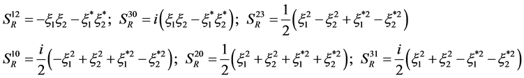
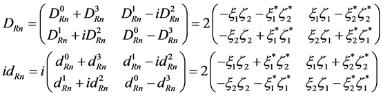
We got with the 8 real parameters of the wave of the electron [4] tensorialdensities². Now with 12 real parameters tensorial densities are awaited. We shall need most of them, so the first part of this study reviews these 78 densities.

In the case of the electron alone the wave equation comes from a Lagrangian density and this is true both with the nonlinear homogeneous equation and with its linear approximation. The difference between these two densities is in the mass term. We got an invariant form for both equations. Since there are 8 real parameters, the wave equation is equivalent to 8 equations. The real one is the cancellation of the Lagrangian density, and another one is the conservation of the current of probability.

It is well known that the electro-weak theory has a problem with the mass term of the Dirac equation, because this term links the left spinor and the right spinor that behave differently in the electro-weak gauge. Then this part of the standard model begins with an electron without mass term and a complicated model of symmetry spontaneously broken is necessary to get a mass term. The aim of this article is to study a wave equation with a mass term that is both relativistic invariant and gauge invariant under the electro-weak gauge group. This was previously thought as impossible.

An invariant form of this wave equation also exists; the Lagrangian density is the real part of this invariant form. We get the wave equation by the Lagrangian mechanism. The conservation of the total current is one of the numeric equations equivalent to the invariant form. The Dirac equation with mass term is the linear approximation of our wave equation for electron + neutrino when we cancel the wave of the neutrino.

2. Tensors

Each of the three spinors has 4 parameters, and then each gives components of tensors, a spacetime vector (4 components) and a space-time bivector (6 components).

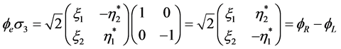
With the only right spinor of the electron

(1.1)

we get the space-time vector and the space-time bivector satisfying³

(1.2)

is a space-time vector, because it satisfies.

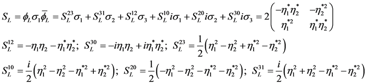
Similarly with the left spinor of the electron

(1.3)

we get the space-time vector and the space-time bivector satisfying

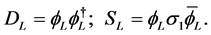(1.4)

It is well known [6] that these currents, are the fundamental ones in the Dirac theory, and the usual currents and are sum and difference of these chiral currents

(1.5)

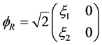
With the left spinor of the electronic neutrino

(1.6)

we get the space-time vector and the space-time bivector satisfying

(1.7)

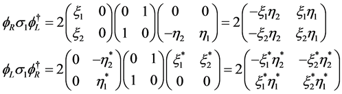
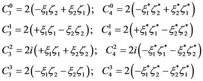
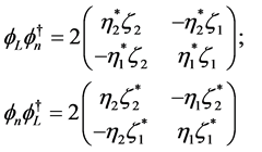
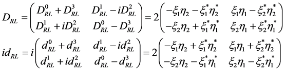
Next with two of these three spinors we can get 16 densities. We begin with and. We let

(1.8)

and are known in the Dirac frame:

(1.9)

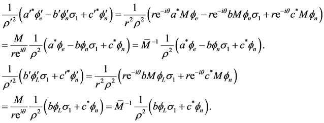
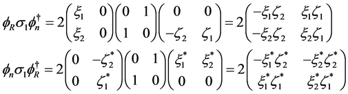
where, are the relativistic invariants of the Dirac theory, and is the Yvon-Takabayasi angle [1] [7] . [5] is the bivector which, with, , and, gives the 16 components of tensors known in the complex Dirac theory. They are those invariant under the electric gauge [3] . and are space-time vectors⁴. To see this, we can consider the form invariance of the Dirac theory. being any complex

matrix, the transformation from the space-time in to itself, which to any associates satisfying

(1.10)

is [4] [5] [8] a Lorentz dilation, product of a Lorentz rotation and of a homothety with ratio satisfying

(1.11)

We get

(1.12)

So is a quantity varying like, a contravariant vector. It is the same for or. We get also

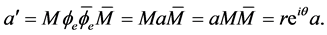(1.13)

Then

(1.14)

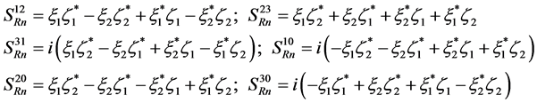
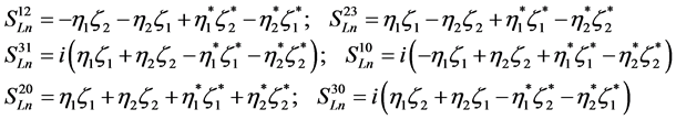
Now with and we let

(1.15)

Vectors and are contravariant vectors, is a bivector. We shall need

(1.16)

Finally with and we let

(1.17)

Vectors and are contravariant vectors, is a bivector. We shall need

(1.18)

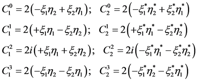
The main invariant term of the electron wave is [1] . Since we get now not only one, but three similar terms, the natural generalization to the wave of the electron and its neutrino is⁵

(1.19)

3. Getting the Wave Equation

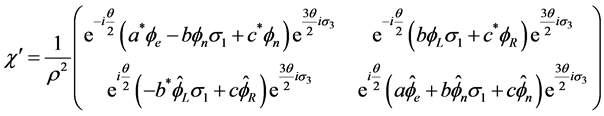
Since this invariant term is the generalization of the invariant mass term of the electron wave, since this term is the mass term of the Lagrangian density [1] , the Lagrangian density of the wave of the electron and its neutrino is the real scalar part of

(2.1)

where, is the reverse and is the covariant derivative satisfying

(2.2)

Projectors satisfy

(2.3)

Noting they satisfy

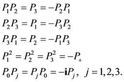(2.4)

Operators are then generators of the Lie group of electro-weak interactions. We shall use

(2.5)

With and. The last equality (2.5) comes from:

(2.6)

which results from our choice [1] of Dirac matrices:

(2.7)

and we get

(2.8)

With (2.2) we get

(2.9)

which gives

(2.10)

Next we get, with

(2.11)

From (2.8) and (2.9) we get with

(2.12)

Next we get, with

(2.13)

We then get

(2.14)

We next get

(2.15)

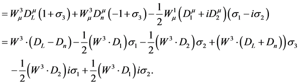
With our matrix representation (2.7) of the space-time algebra, the real part of a multivector is the real part of the scalar part of the matrix. Therefore we get

(2.16)

Next we get

(2.17)

From (2.10) and (2.14) we get

(2.18)

which gives

(2.19)

We next get

(2.20)

For (2.17) we have

(2.21)

And for (2.19) we have

(2.22)

(2.23)

(2.24)

Therefore the Lagrangian density is

(2.25)

The Lagrange equation gives

(2.26)

The Lagrange equation 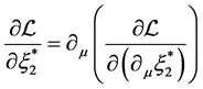gives

(2.27)

Together these equations read

(2.28)

Multiplying by we get

(2.29)

Since and this also reads

(2.30)

then using the conjugation we get

(2.31)

The Lagrange equation 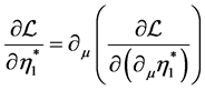gives

(2.32)

The Lagrange equation 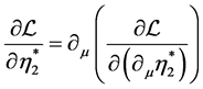gives

(2.33)

Together these equations read

(2.34)

Multiplying by this reads

(2.35)

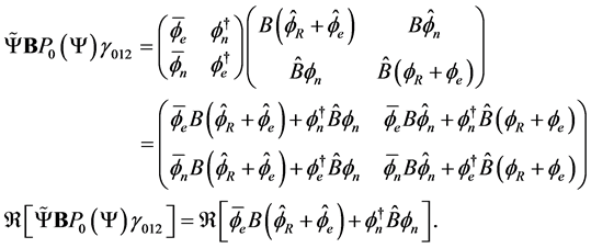
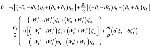
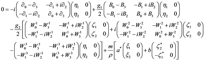
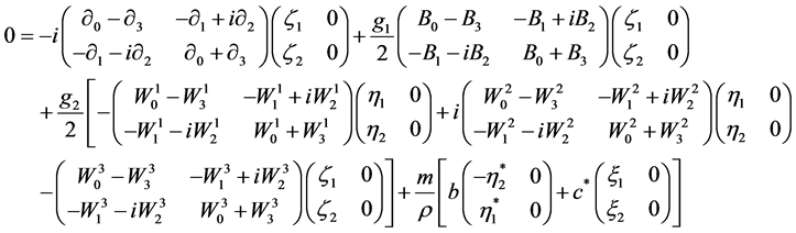
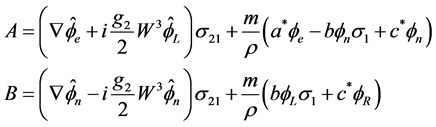
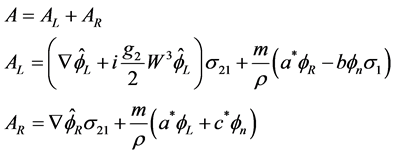
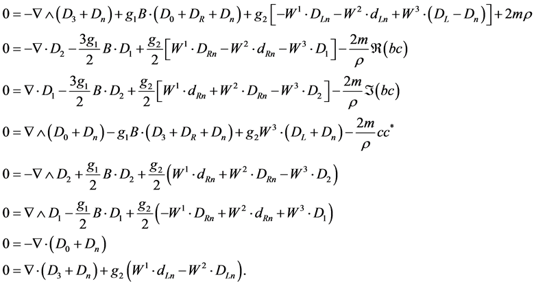
Adding (2.31) and (2.35) we get the wave equation

(2.36)

Without its mass term, this equation is the wave equation of the electron in the electro-weak theory [1] (6.57). The great difference is that there is now a mass term, and since the Lagrangian density is both relativistic and gauge invariant, we shall see that the wave equation with mass term conserves these invariant properties. The Lagrange equation gives

(2.37)

The Lagrange equation gives

(2.38)

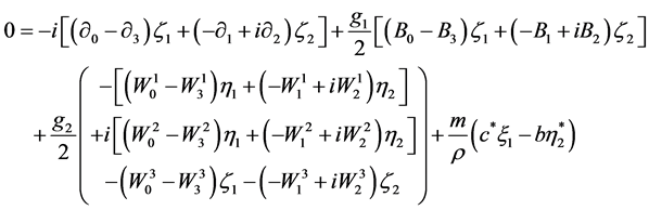
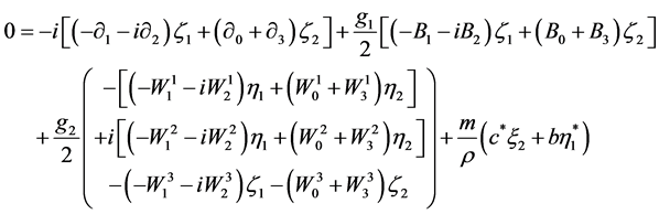
Together these equations read

(2.39)

Multiplying by this reads

(2.40)

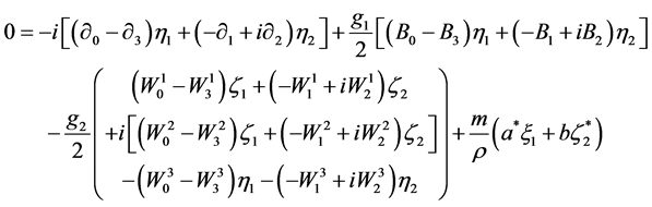
Without the mass term, this equation is the wave equation of the electronic neutrino in the electro-weak theory [1] (6.58). Following backwards the calculation from (2.10) to (2.15) we can see that the system (2.36) (2.40) is equivalent to the wave equation

(2.41)

where

(2.42)

or to the invariant equation

(2.43)

Since this wave equation is not exactly our starting one, we must explain how this equation has exactly the Lagrangian equation as real part. We shall next prove the relativistic invariance and the gauge invariance of this wave equation under the electro-weak gauge group.

4. Invariances

With (2.2) and (2.42) we get

(3.1)

We get

(3.2)

Therefore the Lagrangian density (2.25) is also the real part of the invariant form (2.43) of the wave equation. The value of is more simple because we get

(3.3)

We now review the form invariance of this wave equation; next we shall prove its gauge invariance.

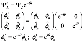
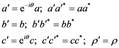
4.1. Form Invariance

Under the multiplicative Lie group made of any invertible matrix satisfying (1.10) We got [1] [3]

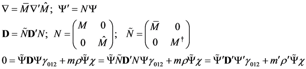(3.4)

And we shall get the form invariance of the wave equation if and only if

(3.5)

From (1.13), (1.16), (1.18) we get with (1.11)

(3.6)

This gives (3.5) since

(3.7)

And the wave equation is form invariant under then it is relativistic invariant.

4.2. Gauge Invariance-Group Generated by P₀

We shall use a convenient form of the projector (proof in [1] B p.143)

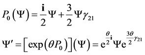(3.8)

We have proved ([1] (B.14)) that

(3.9)

Equation (3.8) reads

(3.10)

This gives

(3.11)

And we get

(3.12)

We then get for:

(3.13)

We must study

(3.14)

We get

(3.15)

and similarly

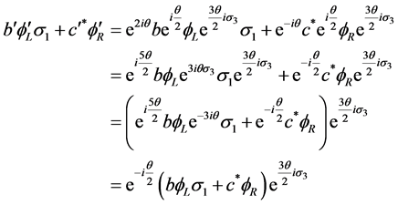(3.16)

This gives

(3.17)

which reads

(3.18)

and we finally get

(3.19)

We may then say that the wave equation is gauge invariant under the gauge transformation generated by.

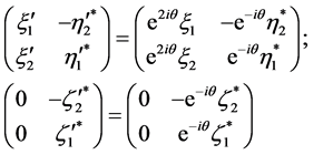
4.3. Gauge Invariance-Group Generated by P₃

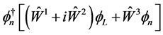
This generator acts only upon left waves: we get

(3.20)

And with left waves we get

(3.21)

That reads

(3.22)

We then get for:

(3.23)

The covariant derivative is here reduced to

(3.24)

We let

(3.25)

We get

(3.26)

Only the left column of is not null, and the result for is simple:

(3.27)

For, which has a left and a right column, we note:

(3.28)

We then get

(3.29)

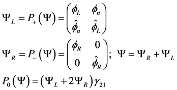
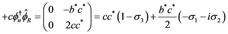
Since the same matrix multiplies the differential part and the mass part of the wave equation, we may say that this equation is invariant under the gauge generated by. We must remark that, even if the wave has value in the Clifford algebra of space-time, it is much easier to use its components in the Clifford algebra of space to get the gauge invariance. The Clifford algebra of space-time is too much symmetric to be the true frame for a gauge invariance which separates completely left and right waves.

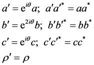
4.4. Gauge Invariance-Group Generated by P₁

This generator also acts only upon left waves: we get And with left waves we get

(3.30)

which reads with and

(3.31)

We get for

(3.32)

The covariant derivative is now reduced to

(3.33)

We let

(3.34)

We get

(3.35)

As previously, for, which has a left and a right column, we note:

(3.36)

We then get

(3.37)

Since the mass term is changed exactly in the same way that the differential term we can say that this wave equation is gauge invariant under the gauge generated by. Now it is not necessary to study, since. We have then proved both the form invariance and the gauge invariance of the wave equation (2.43) under the Lie group generated by.

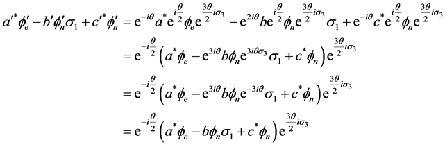
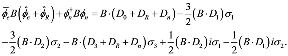
5. Conservative Current

We start from (2.36) and its conjugated equation:

(4.1)

and from (2.40) and its conjugated equation

(4.2)

The differential term of (2.44) is

(4.3)

Then (2.43) reads, which is equivalent to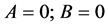. To get the first equation we multiply

(2.36) on the left side by and (4.2) by, this gives

(4.4)

We shall use

(4.5)

We got in [1] (A.18), for any space-time vector, the following equality:

(4.6)

Then the first part of (4.5) reads

(4.7)

Since the second part of (4.5) satisfies

(4.8)

It is a pseudo-vector in space-time and we let

(4.9)

This gives

(4.10)

Similarly we let

(4.11)

which gives

(4.12)

Next we get, with Appendix A:

(4.13)

This gives

(4.14)

We also need

(4.15)

We get with Appendix A:

(4.16)

which gives

(4.17)

We get also with Appendix A:

(4.18)

Since the mass term satisfies (3.2) the wave equation (4.4) is equivalent to the system:

(4.19)

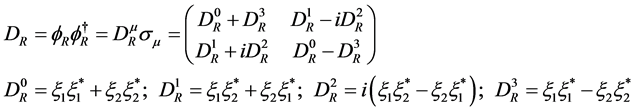
A conservative current exists: it is the total current where is the current of probability in the case of the alone electron, and is the isotropic current of the neutrino. Now these currents are not separately conservative, only the total current is conservative. The calculation is similar for. We get

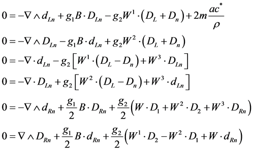(4.20)

6. Concluding Remarks

The conservative law is obviously the simplest equation in (4.19). Contrarily to the case of the electron alone, where is also a conservative current [4] , we get here only one conservative current. When the electron is alone, the conservative current is interpreted as the probability density of presence of the electron. It is really the relativistic generalization of the probability density of the Schrödinger wave. But it is nonsense to think the same for the current, since we have here both an electron and its neutrino.

The mass term of (2.43) replaces by. This is enough to get a wave equation both form invariant and gauge invariant. To get this important novelty in the electro-weak gauge theory, the use of the Clifford algebra of the physical space is essential. It should be impossible to get this using only the algebra of Dirac matrices or the Clifford algebra of space-time. The physical reason is the difference between left and right waves.

We previously studied [9] a wave equation for the electron, with a mass term similar to the mass term obtained here to account for the electron and its neutrino. Another difference between this study and the present one is the role of the Lagrangian density. In the case of the electron alone, or here, the link between the Lagrangian density and the wave equation is double: the Lagrangian density is obtained from the real part of the invariant wave equation, and the wave equation is obtained from the Lagrange equations. Developing the first equation (4.19) and using (2.25) we can see that the first equation (4.19) is. In [9] , we studied a case, which could be extended to the present study, where this double link is cut. The Lagrangian density is again obtained from the real part of the invariant wave equation, but the wave equation cannot be obtained from the Lagrange equations.

The formalism with Dirac matrices ([1] (6.74)) uses and, but we prefer and: because they are true space-time vectors, because the term is here not the usual of quantum fields, generator of the electric gauge, but the of the chiral gauge. Moreover calculations are more complicated with.

When we cancel, we get,; the wave equation is reduced to the homogeneous nonlinear equation previously studied [1] [3] . This equation has the Dirac equation as linear approximation and in the case of the H atom, a set of orthonormal solutions exists with a angle everywhere defined and small. It is exactly the sufficient condition allowing the Dirac equation to approximate our nonlinear homogeneous wave equation. The mass term that we obtained here is also available for the magnetic monopole studied in [1] and [6] [7] [10] .

References

Appendix A

The space-time vector satisfies

(5.1)

The space-time bivector satisfies

(5.2)

(5.3)

The space-time vector satisfies

(5.4)

The space-time bivector satisfies

(5.5)

(5.6)

The space-time vector satisfies

(5.7)

The space-time bivector satisfies

(5.8)

From (1.8) we get (1.9) and

(5.9)

Next we use

(5.10)

And since and we get from (2.60) in [1] :

(5.11)

We have

(5.12)

and with (5.10) we get

(5.13)

which gives

(5.14)

(5.15)

Comparison with (A.17) to (A.20) and with (A.23) to (A.26) in [5] proves that

(5.16)

We let

(5.17)

which gives

(5.18)

Next from (1.17) we get (1.18) and

(5.19)

which gives, with notations similar to (5.5)

(5.20)

We have

(5.21)

and with (1.17) we get

(5.22)

which gives

(5.23)

(4.24)

We let

(5.25)

which gives

(5.26)

Finally from (1.15) we get (1.16) and

(5.27)

which gives, with notations similar to (5.5)

(5.28)

We have

(5.29)

and with (1.15) we get

(5.30)

which gives

(5.31)

(5.32)

We let

(5.33)

which gives

(5.34)

NOTES

¹A complete introduction to this mathematical tool was made in -.

²Only 16 were known with the Dirac formalism.

³A detailed calculation of components is in Appendix A.

⁴If we get, and.

⁵We recall that is an orthogonal mobile basis in space-time, with and,.

References

- Daviau, C. and Bertrand, J. (2014) New Insights in the Standard Model of Quantum Physics in Clifford Algebra. http://hal.archives-ouvertes.fr/hal-00907848
- Daviau, C. and Bertrand, J. (2014) Nouvelle approche du modele standard de la physique quantique en algebre de Clifford, JePublie.
- Daviau, C. (2013) Advances in Imaging and Electron Physics, 179, 1-136. http://dx.doi.org/10.1016/B978-0-12-407700-3.00001-6
- Daviau, C. (2012) Nonlinear Dirac Equation, Magnetic Monopoles and Double Space-Time, CISP, Cambridge (UK).
- Daviau, C. (2012) Double Space-Time and more, JePublie.
- Lochak, G. (1983) Annales de la Fondation Louis de Broglie, 8, 345-370.
- Lochak, G. (1985) International Journal of Theoretical Physics, 24, 1019-1050. http://dx.doi.org/10.1007/BF00670815
- Daviau, C. (2005) Annales de la Fondation Louis de Broglie, 30, 409-428.
- Daviau, C. and Bertrand, J. (2013) Annales de la Fondation Louis de Broglie, 38, 57-81.
- Lochak, G. (1985) The Symmetry between Electricity and Magnetism and the Wave Equation of a Spin 1/2 Magnetic Monopole. Proceedings of the 4th International Seminar on the Mathematical Theory of Dynamical Systems and Microphysics, Udine, 4-13 September 1985, 107-131.