Journal of Modern Physics
Vol.3 No.5(2012), Article ID:19246,15 pages DOI:10.4236/jmp.2012.35051
Study of the Interactions between Particles Based in Paraquantum Logic
1Group of Applied Paraconsistent Logic, Santa Cecília University, Santos, Brazil
2Institute for Advanced Studies, University of São Paulo, São Paulo, Brazil
Email: inacio@unisanta.br
Received January 25, 2012; revised February 10, 2012; accepted March 13, 2012
Keywords: Paraconsistent Logic; Paraquantum Logic; Classical Physic; Relativity Theory; Quantum Mechanics
ABSTRACT
Paraquantum Logic (PQL) has its origins in the fundamental concepts of the Paraconsistent Annotated Logic (PAL) whose main feature is to be capable of treating contradictory information. In this work we presented a study of application of the PQL in resolution of phenomena of physical systems that involves the interactions between physical bodies or particles. Initially is considered that each particle or physical body that is in the physical world has a representative Lattice in the Paraquantum world. From this consideration is made a study of the phenomena of Paraquantum Entanglement modeling the interaction between particles based in fundamental concepts of the Paraquantum Logic. The mathematical relationships of representative Lattices of the Paraquantum Logic originate models with values that are identified with some physical constants. In this work these paraquantum values are identified with the Universal constant of Gravity, proposed by Newton, and the constant K, that relates the Interaction Force in charged particles in the Coulomb’s Law. The results showed that the Paraquantum Logical Model elaborated starting from the fundamental concepts of the Paraquantum Logic (PQL) is adequate to support theories based in a Paraquantum Universe built by an infinite amount of Lattices and forming a Paraquantum net of infinite dimensions.
1. Introduction
The researches developed in Physical science have the main objective to find models capable to simulate with precision our reality. However, in many cases, the expected results are not reached because the extracted signals of information of the real world are incomplete and contradictory.
When we worked with the Classic Physics, the uncertainties, the ambiguities and inconsistencies in the extracted information of the real world cause great difficulties for the creation of efficient models to simulate phenomena of real physical systems. Because of these problems many researches are being developed to find models based on non-Classic Logics. A Paraconsistent Logic (PL) is a non-classical logic which revokes the principle of non-Contradiction and admits the treatment of contradictory information in its theoretical structure [1-4]. The real applications of the PL in programming of computation systems began with an interpretative form that it used annotations, and, for that reason, the PL passed to be denominated of Paraconsistent Annotated Logic (PAL).
The Paraconsistent Annotated Logics with annotation of two values (PAL2v) [3,4] is a class of Paraconsistent Logics particularly represented through a Lattice of four vertices and from its foundations the Paraquantum Logics PQL was created [5].
According to [5] we can obtain through the PAL2v a representation of how the annotations or evidences express the knowledge about a certain proposition P. Considering that μ is the Favorable Degree of evidence and λ is Unfavorable Degree of evidence, then the symbol P(μ, λ) can be read in the following way:
Let be P(m, l) a Paraconsistent Logical Signal (see [4,5]) where the annotation is composed by favorable degree of evidence μ and by unfavorable degree of evidence l and assigned to a proposition P. The logical negation of P is defined as: 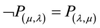
PT = P(1, 1) → intuitive reading that P is inconsistent.
Pt = P(1, 0) → intuitive reading that P is true.
PF = P(0, 1) → intuitive reading that P is false.
P^= P(0, 0) → intuitive reading that P is Indeterminate.
In the internal point of the lattice which is equidistant from all four vertices, we have the following interpretation: PI = P(0.5, 0.5) → intuitive reading that P is undefined.
With the values of x and y that vary between 0 and 1 and being considered in an Unitary Square on the Cartesian Plane (USCP) we can get linear transformations for a Lattice k of analogous values to the associated Lattice τ of the PAL2v [5]. We obtain the following final transformation:
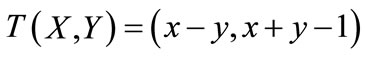 (1)
(1)
According to the language of the PAL2v we have:
x = μ → is the Favorable evidence Degree y = λ → is the Unfavorable evidence Degree.
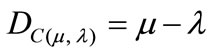
The first coordinate of the transformation (1) is called Certainty Degree DC. So, the Certainty Degree is obtained by:
 (2)
(2)
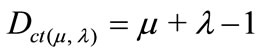
The second coordinate of the transformation (1) is called Contradiction Degree Dct. So, the Contradiction Degree is obtained by:
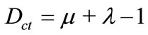 (3)
(3)
The second coordinate is a real number in the closed interval [–1,+1]. The y-axis is called “axis of the contradiction degrees”.
Since the linear transformation T(X,Y) shown in (1) is expressed with evidence Degrees μ and λ, then from (2), (3) and (1) we can represent a Paraconsistent logical state eτ into Lattice τ of the PAL2v [5,6], such that:
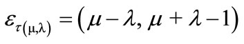 (4)
(4)
or
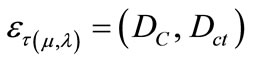 (5)
(5)
where:
eτ is the Paraconsistent logical state.
DC is the Certainty Degree obtained from the evidence Degrees μ and λ.
Dct is the Contradiction Degree obtained from the evidence Degrees μ and λ.
Figure 1 shows the Lattice of the LPA2v and where is obtained a point (DC, Dct) where DC = ƒ(μ,λ) and Dct = ƒ(μ,λ) which represents a Paraconsistent logical state ετ.
The main concepts and foundations of the logic LPA2v can be found in [5] and in [6]. Through the resultant equations of analyses in the PAL2v Lattice the principles of the Paraquantum Logic was created. This paper is organized in the following way: Section 2 shows the
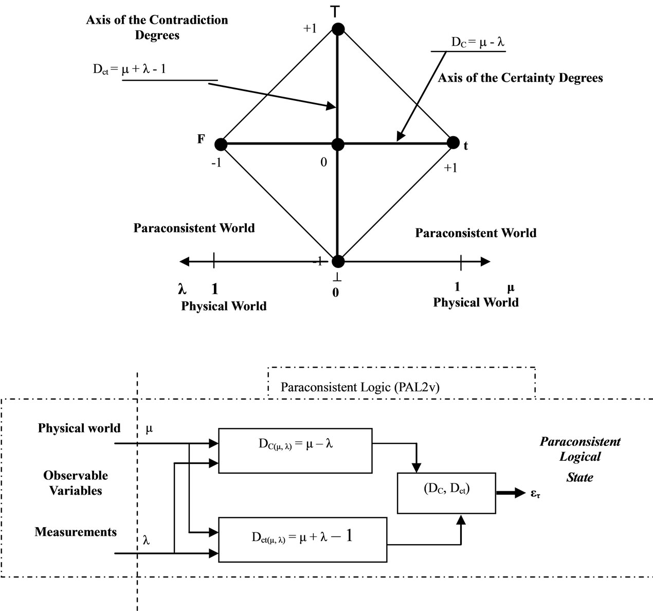
Figure 1. The lattice of the LPA2v and the Paraconsistent logical state ετ.
main concepts of the Paraquantum Logic, Section 3 a Paraquantum Logical model for quantization of values is proposed. In the Section 4 the phenomenon of Paraquantum Logical Entanglement and the effects of interactions among particles are studied with details and finally, the conclusion is presented in Section 5.
2. The Paraquantum Logic PQL
Under certain conditions the results obtained from the LPA2v model changed through leaps or unexpected variations [7]. This behavior in the resulting values demonstrates that the application of its foundations offered results strongly connected to the ones found in modeling of phenomena studied in quantum mechanics (see [7,8]). Following this reasoning line a Paraquantum logical state ψ is created on the lattice of the PQL as the tuple formed by the certainty degree DC and the contradiction degree Dct [9,10]. Both values depend on the measurements perfomed on the Observable Variables in the physical environment which are represented by μ and λ [10,11]. This way, we can express (2) and (3) in terms of μ and λ obtaining:
 (6)
(6)
 (7)
(7)
And a Paraquantum function y(Py) is defined as the Paraquantum logical state y:
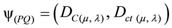 (8)
(8)
For each measurement performed in the physical world of μ and λ, we obtain a unique duple  which represents a unique Paraquantum logical state ψ which is a point of the lattice of the PQL [10]. On the vertical axis of contradictory degrees, the two extreme real Paraquantum logical states are:
1) The contradictory extreme Paraquantum logical state which represents Inconsistency T:
ψT 
2) The contradictory extreme Paraquantum logical state which represents Undetermination ^:
ψ^ 
On the horizontal axis of certainty degrees, the two extreme real Paraquantum logical states are:
3) The real extreme Paraquantum logical state which represents Veracity t:
ψt 
4) The real extreme Paraquantum logical state which represents Falsity F:
ψF .
.
A Vector of State P(ψ) will have origin in one of the two vertexes that compose the horizontal axis of the certainty degrees and its extremity will be in the point formed for the pair indicated by the Paraquantum function y(Py) [10].
If the Certainty Degree is negative (DC < 0), then the Vector of State P(ψ) will be on the lattice vertex which is the extreme Paraquantum logical state False: ψF = (–1, 0).
If the Certainty Degree is positive (DC > 0), then the Vector of State P(ψ) will be on the lattice vertex which is the extreme Paraquantum logical state True: ψt = (1, 0).
If the certainty degree is nil (DC = 0), then there is an undefined Paraquantum logical state ψI =(0.0, 0.0).
The Vector of State P(ψ) will always be the vector addition of its two component vectors:
 Vector with same direction as the axis of the certainty degrees (horizontal) whose module is the complement of the intensity of the certainty degree:
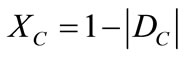
 Vector with same direction as the axis of the contradiction degrees (vertical) whose module is the contradiction degree:
Given a current Paraquantum logical state ψcur defined by the duple  then we compute the module of a Vector of State P(ψ) as follows:
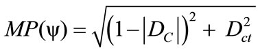 (9)
(9)
where:
DC = Certainty Degree computed by (6)
Dct = Contradiction Degree computed by (7).
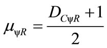
The real Certainty Degree (DCψR) is the value of the certainty degree without the effect of the contradiction. Using (9) which is for computing the module of a Vector of State P(ψ), we have:
1) For DC > 0 the real Certainty Degree is computed by:
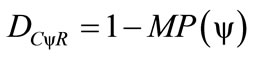 (10)
(10)
Therefore:
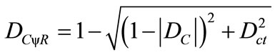 (11)
(11)
2) For DC < 0, the real Certainty Degree is computed by:
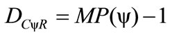 (12)
(12)
Therefore:
 (13)
(13)
where:
DCψR = real Certainty Degree.
DC = Certainty Degree computed by (6).
Dct = Contradiction Degree computed by (7).
3) For DC = 0, then the real Certainty Degree is nil:
The intensity of the real Paraquantum logical state is computed by:
 (14)
(14)
The inclination angle ay of the Vector of State is computed by:
 (15)
(15)
2.1. Uncertainty Paraquantum Region
The propagation of the superposed Paraquantum logical states ysup through the lattice of the PQL happens due to the continuous measurements performed on the Observable Variables in the physical world [10,11]. Since the Paraquantum analysis deals with favorable and unfavorable evidence degrees μ and l of the measurements performed on the physical world, these variations affect the behavior and propagation of the superposed Paraquantum logical states ysup on the lattice of the PQL.
When the module of the Vector of State MP(ψ) = 1, this vector will represent the maximal fundamental superposed Paraquantum logical states ψsupfmax which has real certainty degrees zero. The maximum Contradiction Degree for this condition is when the Vector of State P(ψ) forms an angle of 45˚ with the horizontal axis of certainty degrees.
When the module of the Vector of State is of larger value than the unit MP(ψ) > 1, means that the Paraquantum logical state ψ are in an uncertainty region. The Paraquantum logical states into limits of the Region of Uncertainty are identified with Factors of maximum limitation of transition [10]. These factors are:
1) The factor of Paraquantum limitation False/inconsistent—hQyFT.
 º hQyFT
2) The factor of Paraquantum limitation True/inconsistent—hQytT.
 º hQytT
3) The factor of Paraquantum limitation False/undetermined—hQyF^.
 º hQyF^
4) The factor of Paraquantum limitation True/undetermined—hQyt^.
 º hQyt^
The unbalanced contradictory Paraquantum logical state ψctru is the one located on the lattice of states of the PQL where there is a condition of opposite signs between the Certainty Degree (DC) and the real Certainty Degree (DCψR).
2.2. The Paraquantum Factor of Quantization hψ
When the superposed Paraquantum logical state ysup propagates on the lattice of the PQL a value of quantization for each equilibrium point is established. This point is the value of the contradiction degree of the Paraquantum logical state of quantization yhy [10] such that:
 (16)
(16)
where: hy is the Paraquantum Factor of quantization.
The factor hy quantifies the levels of energy through the equilibrium points where the Paraquantum logical state of quantization yhy, defined by the limits of propagation throughout the uncertainty of the PQL, is located.
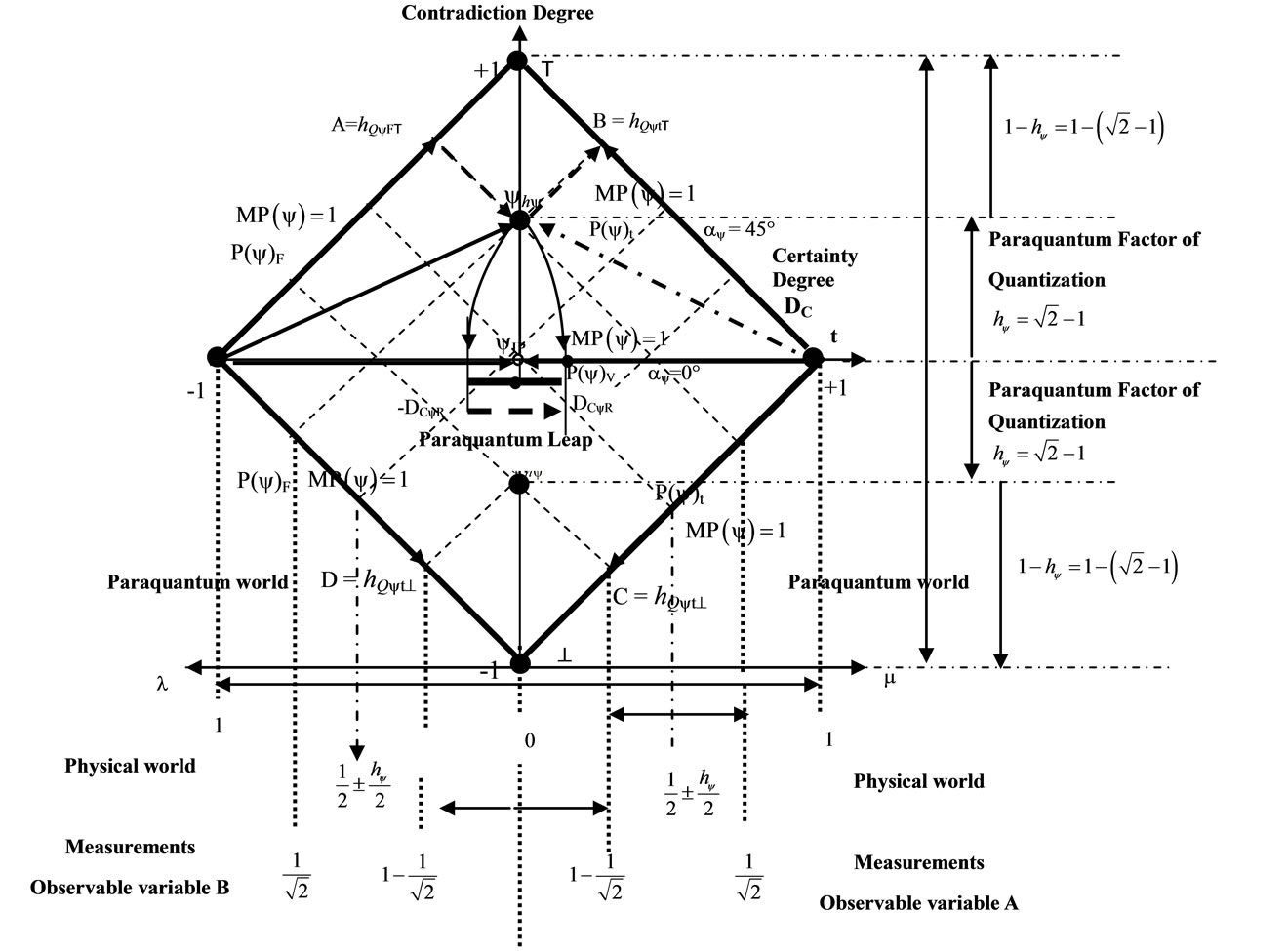
Figure 2(a) shows the Paraquantum Factor of quantization (hy) and the interconnections between the factors and its characteristics, in which they delimit the Region of Uncertainty in the Lattice of PQL.
2.3. The Paraquantum Leap
In a process of propagation of Paraquantum logical state y, we have that in the instant that the superposed Paraquantum logical state ysup reaches the representative points of the limiting factors of the uncertainty region of the PQL, the Certainty Degree (DC) remains zero but the real Certainty Degree (DCyR) will be increased or decreased from zero and this difference corresponds to the effect called of the Paraquantum Leap [10,11]. In order to completely express it, we have to take into account the factor related to the Paraquantum Leaps which will be added to or subtracted from the Paraquantum Factor of quantization [10] such that:
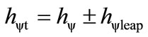 (17)
(17)
where, from Figure 2 we can make the calculations:
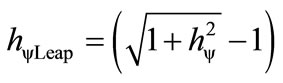 (18)
(18)
So, the Factor of Paraquantum Quantization in its complete or total form which acts on the quantities is:
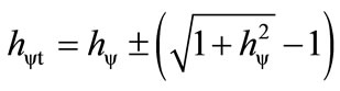 (19)
(19)
Being:  the total Factor of Paraquantum Quantization at the time of arrival of the Superposed Paraquantum Logical state ψsup at the point where the Paraquantum Logical state of Quantization ψhψ is located.
 is the total Paraquantum Factor of Quantization at the departure of the Superposed Paraquantum Logical state ψsup at the point where the Paraquantum Logical state of Quantization ψhψ is located. Figure 2(b) shows the effect of the Paraquantum Leap in the quantization of values when the Superposed Paraquantum Logical states ysup reach the point where is the Paraquantum Logical state of Quantization ψhψ on the PQL Lattice.
2.4. Newton Gamma Factor
In the International System of units (SI), to express the value of force F in a unit of Newton, an adjustment on the value of mass is necessary [12]. Doing such comparisons and analogies between the International unit Systems (SI) and the British System we obtain for the proportionality factor k in the equation which expresses Newton’s second law (see [11,12]):
 in the British System.
 in the International System of units (SI).
Given the importance of the Factor , which will be largely used in the equations of the PQL, its value is called Newton Gamma Factor whose symbol is
  [11].
[11].
Therefore, in order to apply classical logics in the Paraquantum Logical model, the Newton Gamma Factor is .
.
2.5. Paraquantum Gamma Factor γPψ
The Lorentz Factor  can be identified in the infinite Power Series of the binomial expansion [13,14] related to the series obtained from consecutively applying the Newton Gamma Factor
  (see [11]). In the paraquantum analysis [10,11] we define a correlation value called Paraquantum Gamma Factor
  such that:
 (20)
(20)
where:
 is the Newton Gamma Factor:
 is the Lorentz factor which is:
Using the Paraquantum Gamma Factor  allows the computations, which correlate values of Observable Variables to the values related to quantization through the Paraquantum Factor of quantization hψ [10,11].
3. Paraquantum Logical Model Applied in Calculations of Quantization of Values of Physical Quantities
The quantitative analysis on the PQL Lattice defines a quantitative value QValor of any physical quantity, which can be represented on the horizontal axis of the certainty Degrees and on the vertical axis of the contradiction degrees of the PQL Lattice. Since the maximum value is normalized on the PQL Fundamental Lattice [10,11], considering the Paraquantum factor of quantization only, we can write: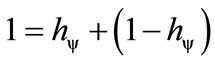 .
.
Doing so, in the PQL Fundamental Lattice the unitary value of the quantization is equivalent to a paraquantum quantization represented in the Paraquantum Logical state ψhψ added to the value of its complement. We have:
 (21)
(21)
where:  is the value of the total amount represented on the unitary axis of the PQL Fundamental Lattice.
Equation (21) shows that the maximum amount of any quantity in the physical environment is composed by two quantized fractions where: one is determined on the Paraquantum Logical state of Quantization ψhψ by the Paraquantum Factor of quantization hψ and the other is determined by its complement (1 – hψ). When the Paraquantum Gamma Factor  is applied on the paraquantum quantities, besides correlating the paraquantum values to the physical environment, it also works as a factor of expansion or contraction of the PQL Lattice.
Representation of Levels of Energy in the Lattice of PQL
By representing the involved Energy in the Paraconsistent Logical Model as being the energy amount represented on the vertical axis of contradiction, we can initially make an analogy with Equation (21) which defines the amount on the PQL Fundamental Lattice in its static form. So, for the Energy, the equation is:
 (22)
(22)
When related to the physical environment, we have:
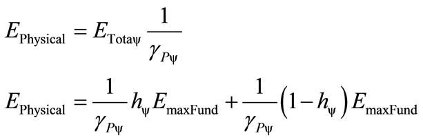 (23)
(23)
The value of the quantity of Energy of Propagation quantized, when considered in its static form, therefore, without considering the effect of the Paraquantum Leap,
 (a)
(a) (b)
(b)
Figure 2. (a) The paraquantum factor of quantization hy related to the evidence degrees obtained in the measurements of the observable variables in the physical world; (b) The value of the paraquantum leap on the paraquantum logical state of quantization yhy .
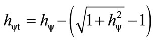
is computed by:
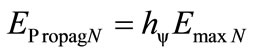 (24)
(24)
where: hψ is the Paraquantum Factor of quantization.
 is the Energy transformed in the propagation of the Paraquantum Logical state of the extreme Vertex False until it reaches the point where the Paraquantum Logical state of Quantization ψhψ is located.
 is the maximum Energy on the level N of the transition frequency.
Since the process of transformation of energy is dynamical, we must consider the effects of Paraquantum Leaps on the Paraquantum Logical Model. So, the total energy transformed, that will constitute the Superposed Fundamental Lattice, will be obtained with adding the Inertial or Irradiating Energy Eirr that appears due to the effects of Paraquantum Leaps. Being the Factor of Quantization on the Paraquantum Leap defined on Equations (17) and (18), the Inertial or Irradiating Energy is expressed by:
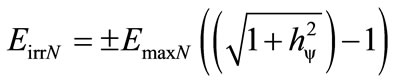 (25)
(25)
So, the total energy transformed at the equilibrium point of the Lattice of the PQL is computed by:
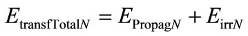 (26)
(26)
or:
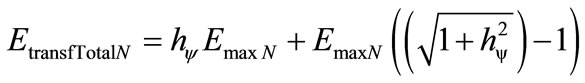 (27)
(27)
So, Equation (22) is rewritten as follows:
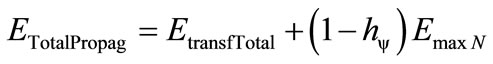 (28)
(28)
or as follows:
 (29)
(29)
Or, in a more complete way, as follows:
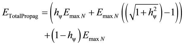 (30)
(30)
From Equation (23)
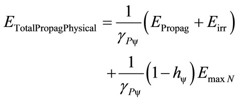 (31)
(31)
The second term of Equations (30), (31) is the complemented value which represents the remaining maximum energy, therefore, it is that amount of energy capable of still being transformed. So, the remaining energy ERestmax is the one which outcomes the value which will be represented on the vertical and horizontal axis of the Lattice of the PQL.
4. The Paraquantum Logical Entanglement and the Interaction between Particles
The phenomenon of Paraquantum Logical Entanglement is inherent to the foundations of Paraquantum Logics, where the PAL2v is originated and where the analysis is only possible using two representing values of information (see [5]). Therefore, for the paraquantum analysis there will always be an entanglement of information from evidences about the proposition to be analyzed.
Considering the formalism of a Paraconsistent logic of two values (PAL2v) [4-6], the concept of Paraquantum logical state ψ on a system in a given instant can only be represented by the Paraquantum logical entanglement of the two Evidence Degrees λ and μ, which are obtained from measurements of the Observable Variables on the physical environment. So, in the language of the Paraquantum Logics, the entanglement between the favorable Evidence Degree μ and de unfavorable Evidence Degree λ produces the representation of a final Paraquantum logical state ψatual+1 visualized through the Intensity Degree of the Real Paraquantum logical state μψR and computed by Equation (14). On the physical environment an observer visualizes the variations of the Real Certainty Degree DCψR transformed by normalization in Intensity Degree of the Real Paraquantum logical state μψR. So, the Paraquantum logical state ψ is composed by the entanglement of information produced by the measurements of the two Observable Variables, which is studied by the Vector of State P(ψ) which is on the plane of the Lattice of States of the PQL. The disappearing of one of the information sources by momentary obstruction of μ or λ in a process of continuous analysis produces what we can call collapse of the Vector of State P(ψ). In this case all resulting values will be on the axis of the Real Certainty Degrees, for there is no contradiction in the analysis. In this condition there Information Entanglement represents the effects of a classical analysis where no contradictory information is allowed.
4.1. The Paraquantum Logical Entanglement between Two Propositions
After a paraquantum analysis, where the measurements originated from Observable Variable on the physical environment are transformed into Evidence Degrees μ and λ compounding the annotation to assign a logical meaning to the proposition P, we can consider the following real situation:
Consider a special condition which involves a system that was divided in two exactly equal parts but due to behaviors observed on the physical environment, to these two halves there are logically negated propositions. This situation can be studied on the Lattice of States by entangled analysis through PQL where the concepts of entanglement of Paraquantum logical states are used for two simultaneous analysis of a proposition P and its logical negation P.
Being the physical System divided into two identical systems SA and SB, Proposition P1 of SA will be analyzed with its negation P1 of SB. This condition does not change the system physically, however produces the need of two simultaneous Paraquantum analyses: one for proposition P1 and other for its logical negation P1. So, for the paraquantum analyses performed simultaneously about the entanglement phenomenon of Paraquantum logical states, we use the concept of logical negation of the PAL2v where there is the exchange of the favorable Evidence Degree μ with the unfavorable Evidence Degree λ on the annotation.
For a simultaneous Paraquantum analysis on two exactly equal systems with negated propositions, we have the information in the form of a Paraquantum logical entanglement.

If we perform measurements of the Observable Variables under these conditions, we can consider the following situations:
The physical System SA has always Favorable Evidence Degree: μA
The physical System SB has always Favorable Evidence Degree: μB
The physical System SA has always Unfavorable Evidence Degree: λA = μB
The physical System SB has always Unfavorable Evidence Degree: λB = μA
The measurements from the Observable Variables are simultaneously entangled in the two paraquantum analyses. As a result, the value of the Real Evidence Degree DCψRA observed at the physical system SA will always be the complement of the resulting value of the Real Evidence Degree DCψRB observed at the physical system SB.
4.2. Paraquantum Entanglement in the Interaction between Two Equally Physical Bodies or Particles
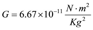
In the process of Paraquantum logical Entanglement of the information from measurements performed on the Observable Variables on the physical environment [15, 16], the paraquantum analysis is performed such that there are two symmetric Lattices where the values of measurements represented through the equality of values μA = λB and μB = λA will simultaneously compound two pairs related to two Paraquantum Logical states ψA = (DC, Dct) and ψB = (–DC, Dct) resulting in Certainty Degrees always with changed signs. For these two analyses the Module of the Vectors of State MP(ψ) will have the same simultaneous variations and the two resulting values of Intensity Degrees of the Real logical state μψRA and μψRB will have symmetry with respect to the Indefinition value 0.5.
In the paraquantum analysis, the entanglement of two Systems takes into account two symmetric Lattices which are in the same Universe of Discourse in only one Fundamental Lattice. Since the variations of the measurements on the physical systems SA and SB occur in the physical environment, they are reflected into the Lattice of States through the values of the Evidence Degrees μ and λ and their intensities depend on the scale or on the Interval of Interest considered. So, every paraquantum analysis in the paraquantum universe is locally performed, being the Proposition logically negated and represented on the side of the opposite Vertices that connects the axis of the certainty degrees. So, since the proposition (P1) of a system is the logical negation of the proposition of the other (P1), a variation in one of the measurements will instantly reflect on the symmetric values of the Intensity Degrees of the Real logical state of these two physical systems being analyzed. In case a Paraquantum Leap occurs due to the contradiction on the measurements from the side such that DC > 0 to the side such that DC < 0 on the physical system SA, then on the physical state SB a Paraquantum Leap will simultaneously occur from the side such that DC < 0 to the side such that DC > 0. Figure 3 shows the entanglement of the information obtained from measurements performed on the Observable Variables on the physical environment S that was divided in two physical systems SA and SB.
4.3. The Paraquantum Entanglement in the Interaction between Two Different Physical Bodies or Particles
The Paraquantum logical entanglement can be studied by considering the Paraquantum Logical Model applied to the effects that appear in the interaction among different physical systems or particles in the physical environment. Since the particles in this case are not equal, we have to take these differences into account in the Paraquantum analysis.
Initially we can consider for this study the interaction between two physical bodies A and B, where body A is represented by its Paraquantum Logical Model A, and this will be a reference. In the existence of the Paraquantum entanglement phenomenon, the presence of the physical body B will affect the Lattice of the PQL which represented the Paraquantum Logical Model of the reference body A such that the effect will be the creation of a Fundamental Lattice through an expansion on the reference Lattice of Body A. The expansion will cover in only one Resulting Fundamental Lattice the reference physical

Figure 3. Paraquantum entanglement of information from measurements performed on observable variables which are linked to two identical physical systems SA and SB, but with propositions logically negated.
body A and the external physical body B. In this condition, for the Lattice of the reference Paraquantum Logical Model, the presence of body B changes the initial values and the paraquantum analysis will produce referenced values through the expansion.
4.4. The Universal Gravitational Constant and the Paraquantum Logic
In the interaction of different physical bodies on the Paraquantum Entanglement, we observe that the values obtained on the Lattice of the Paraquantum Logical Model of the reference body A can be related to the value of the Universal Gravitational constant G [12].
The Universal Gravitation Law proposed by Newton says that all objects are attracted to others with a force directly proportional to the product of their masses and inversely proportional to the square of the distance between their centers. So, the most important physical phenomena of the observable universe are expressed in only one equation, showing that there are no differences between the terrestrial and the celestial physics [13].
In the study of the Paraquantum Entanglement, we observe that this interaction process appears in a natural way, since it is enough to consider a second physical system and a Fundamental Lattice which involves both systems is created. The Paraquantum analysis between two Lattices that represent the Paraquantum Logical Models of Physical Systems shows that the paraquantum Entanglement occurs with the notion of distance and Interaction Force among them. So, the value of a Paraquantum Gravitation Constant can result from Quantization factors due to superposed Paraquantum Logical states which appear through the expansion of the Fundamental Lattice of the PQL. This natural process that occurs on the Paraquantum Logical Model identifies a resulting value of the Paraquantum Factor of quantization very close to the value established as the Universal Gravitational constant. We call this value Paraquantum Gravitational Constant Gψ. For a comparative study of values, first we present how we obtained Newton’s Gravitational Constant G through Kepler’s equations.
4.5. Universal Constant of Gravitation of Newton
The studies that involve concepts of force, movement states and equations of Energy make the Law of Universal Gravitation (UG) of Newton a mathematical tool of great interest to deal with physical phenomena and it was proposed from Kepler’s laws [12]. For the case of circular orbits, the inverse quadratic nature of the centripetal force can be easily computed from Kepler’s third law which is about the planetary movement and the dynamics of the uniform circular movement. According to Kepler’s third law, the square of the period T is proportional to the cube of the greater semi-axis of the ellipse. In the case of the circumference, the greater semi-axis is its own radius R, then the mathematical expression for this statement is:
 (32)
(32)
where: K is the proportionality constant.
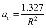
In the study of the uniform circular movement (UCM) the velocity of the moving body does not vary in module, however constantly varies in direction [12]. The moving body has an acceleration which is directed to the center of the course, called normal acceleration whose module is computed by:
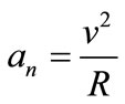 (33)
(33)
Since the velocity v and the radius R in the Uniform Circular Movement have constant values, the module of the centripetal acceleration varies continuously because is directed from the object to the center of the circle.
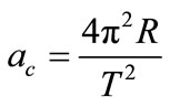 (34)
(34)
Multiplying both sides of the equation again by R2, we have: 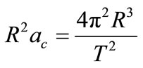
Isolating the square of the period: 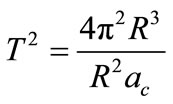
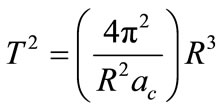
Rewriting, we have:
 (35)
(35)
This equation can be compared to the third Kepler’s law for the study of the movements of celestial bodies, described by Equation (35).
 ↔
↔ 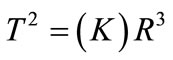
From Equation (35) we obtain an important relation:
 (36)
(36)
In the study of the planets it was observed that the product of acceleration by the square of the radius R appeared with a constant Ks such that: .
.
From where we can isolate the acceleration as follows:
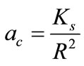 →
→
The dynamics of the uniform Circular Movement (UCM) is such that, in a circular course, the force that we have to apply to the body is equal to the product of its mass by the normal acceleration, therefore from the equation that expresses Newton second law, we obtain:
 →
→
We can compare the equations: 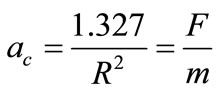
From where we obtain the force computed by:
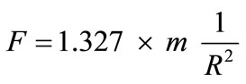
This equation expresses the gravitational force that decreases with the increase of R, known as the Force of the square inverse. According to Newton, the gravitational force performed by the sun on a planet is proportional to the mass of the planet. By Newton’s third law, if the sun performs a force  on a planet, then the planet performs a force
  on the sun, where the moduli of the forces are equal:
 . In order to find the gravitational constant in the study of interaction force between the planets, we must know the masses involved [12,13]. A proportionality constant was established which is independent of any masses such that:

and

and
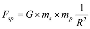
In the interaction between the two masses, each one performs the half of the constant  represented as a gravitational constant G. So, we have the corresponding value of the Universal Gravitational Constant:
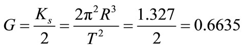
Henry Cavendish (1731-1810) performed the first measurements of G through the well known device called “Cavendish’s Scales”. The value of the Universal Gravitational constant accepted nowadays is [12-15]:
4.6. The Paraquantum Gravitational Constant Gψ
The Paraquantum Gravitational constant Gψ appears on the paraquantum analysis when we make an analogy between the interaction of bodies or particles with the effect of Paraquantum Entanglement.
As an example, we can observe from the following Figure 4 that two bodies can be different in their physical dimensions represented by two Lattices of the PQL where, for the paraquantum analysis, there will always be an interaction between the two bodies in which a unique expanded Fundamental Lattice will be created. According to what was seen, the paraquantum analysis is always performed through a Lattice assigned to the PQL where the properties and forms of propagation of the Paraquantum Logical states ψ are analyzed.
The propagation of the Paraquantum Logical state is characterized by the behavior and variation of the values of the Evidence Degrees extracted from the Observable Variables in the physical environment. The analysis on a Lattice is always done considering a proposition related to one only body. In this analysis, the body or physical system being studied always presents two or more physical quantities which are considered as Observable Variables from where we extract two Evidence Degrees: one favorable and another one unfavorable making reference to the proposition P.
In the practice the Evidence Degrees are normalized values and are in the closed real interval [0,1] where they are extracted from measurements established within an Interval of Interest or Universe of Discourse. So, when a second physical body is found to be considered as a physical system belonging to the Paraquantum analysis, the PQL Lattice receives an expansion action that will cover both bodies in an interactive analysis. This is the effect of Paraquantum Entanglement applied to two bodies that may be different according to what will be considered in this study.
This natural Interaction for the paraquantum analysis causes both physical systems to interact creating a unique new Fundamental Lattice with all characteristics of normalizations and with Quantization factors of the individual Lattice. According to the properties of the PQL, the new Lattice which is created by the interaction of the two bodies is bounded by the Region of Paraquantum Uncertainty. So, the interaction on the physical world between the two particles happens on the action line of the Paraquantum Gamma Factor γψ which delineates new equilibrium points of the new fundamental Lattice.
The following Figure 5 shows this interaction of two individual Lattices and the creation of a unique Fundamental Lattice from where, through a trigonometric process, we can obtain the resulting value of the Quantization Factor. When the values are considered in relation to each one the individual Lattices, the bounds of the new Fundamental Lattice expanded by the interaction of the two physical systems will increase equilibrium points.
This effect causes the resulting value of the Quantization Factor, for the reference taken from the Lattice of each individual physical System, to be an aggregation of values given by:
 (37)
(37)
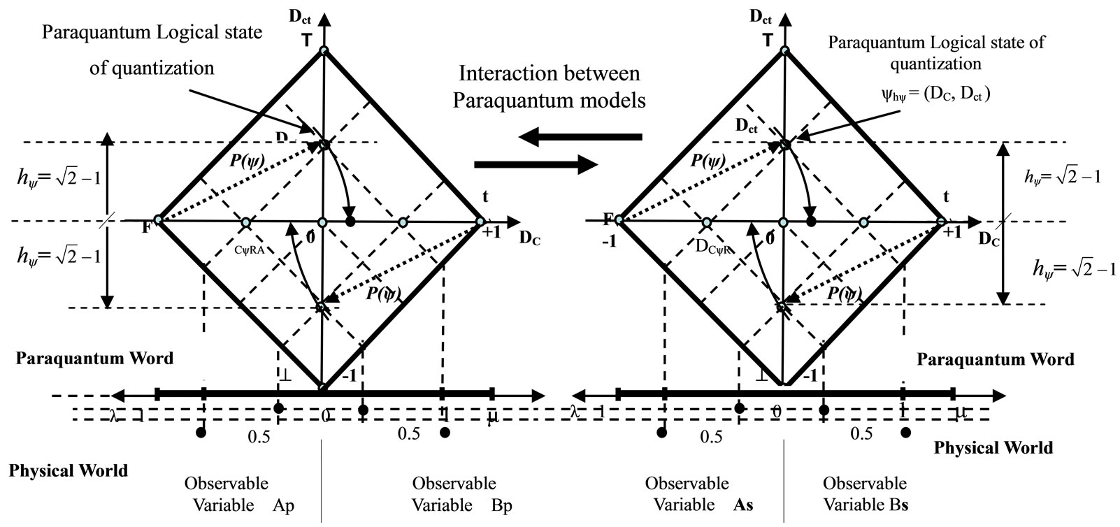
Figure 4. Two Lattices of the PQL representing two different physical systems or an interaction that will mandatorily be analyzed on a unique expanded Lattice.
Figure 5. Both Lattices of the PQL representing two physical systems whose interaction generates a unique expanded Fundamental Lattice.
where:  is the Paraquantum Factor of quantization.
 = Resulting Value of the Paraquantum Factor of quantization expanded by the interaction of the two physical systems computed by the individual Lattice. As:
 , then, computing the value of the Quantization Factor in an aggregation of values obtained by the interaction of the two Lattices, as Equation (37) shows, we have:

→
Being an expansion value due to the interaction caused by the presence of another body in the analysis, we call this value Factor of Constant of Paraquantum Gravitation Gψ, such that for the interaction of two bodies, we have:
 (38)
(38)
Since: , from Equation (38) the value of the constant of Paraquantum Gravitation results:

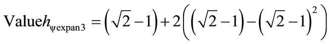
4.7. The Paraquantum Logical Model for Interaction of Several and Different Particles
Through the paraquantum analysis we can study the interaction of particles where the representing Lattices of each physical body are considered in only one set formed by Paraquantum Logical models capable of modeling complex physical systems.
Figure 6 shows the example of the interaction of three systems forming only one expanded Fundamental Lattice such that the study takes into account the Lattice on the left as the referential one.
For this condition, where the reference of values is considered from the Lattice of each individual physical System, we have the resulting value of the Paraquantum Factor of quantization for this type of Paraquantum Entanglement of three Lattices, resulting in an aggregation of values on the vertical axis of the Lattice on the left.
This value shown on the vertical axis of the left-hand side Lattice is computed by:
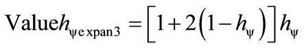 (39)
(39)
where:

Figure 6. The three Lattices of the PQL representing three physical systems whose interaction form a unique Fundamental Lattice expanded.
 is the Paraquantum Factor of quantization.
 = resulting value of the Paraquantum Factor of quantization expanded by the interaction of the three physical systems computed by the individual left-hand side Lattice.
As in the Fundamental Lattice  so the new value of the Paraquantum Factor of quantization obtained by the interaction of the three Lattices according to Equation (39) is:

→
We observe that when we consider the interaction among different particles as an effect of the Paraquantum Entanglement where the value of the Factor of Paraquantum Quantization is obtained in this way, the Paraquantum analysis can be expressed by the notion of distance among the bodies. So, we can make an analogy of the value obtained as the Paraquantum Entanglement of the three Physical Systems with the value of the constant K that related the Interaction Force in charged particles studied with Coulomb’s Law.
4.8. The Paraquantum Universe Model
The analysis of complex physical systems represented by several Lattices forming an interlaced net can be identified as a model of Paraquantum universe. Based in the figures, if the reference Lattice is the Paraquantum Lattice represented to the left of the group, the equation to compute the value on the vertical axis is:
For two Lattices N = 2:


For three Lattices N = 3:

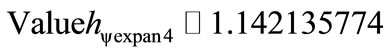
For four Lattices N = 4:
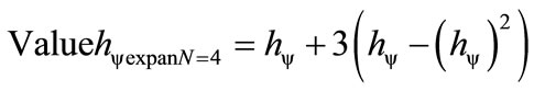

For an amount N of Lattices the equation is:
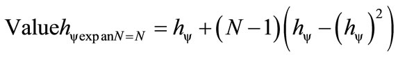 (40)
(40)
 is the Paraquantum Factor of quantization.
 = resulting value of the Paraquantum Factor of quantization expanded by the interaction of N physical systems computed by the individual left-hand side Lattice. where: N is the number of Paraquantum Lattices of the group.
However, when the number of Lattices of the group will be greater that 3 (N > 3) the calculated value will be greater that 1 ( ). This makes with that the reference Lattice of the group is changed and it passes to be the next Lattice to the right.
The idea of the contracted model, where the Fundamental Lattice aggregates or receives smaller Lattices in its inner side, makes us consider a notion of mass or formation of matter in the paraquantum analysis. So, the Paraquantum Entanglement in the analysis of Physical Systems is about the process where, for each pair of Lattices representing two physical bodies, a new third one will be formed as a paraquantum agglutinatoer. So, the agglutinating Lattice will be the reference one and its position will be the middle of the Fundamental Lattice. In this analysis, the value of the Paraquantum Factor of quantization will be expressed in relation to the Fundamental Lattice that will be subject to a contraction process according to what was studied in the Paraquantum Logical Model (see [17,18]).
5. Conclusion
In this paper, we presented a study about the Paraquantum Entanglement covering similar and different systems where the values related to the interaction among bodies or physical particles were established. The obtained results produce large possibilities for new researches where Paraquantum Logics is a good option to serve as a base for models of physical models interconnecting through the paraquantum universe several areas of physics which nowadays have results which are not compatible. The researches about resulting values of the interactions of different bodies in the form of the Paraquantum Entanglement can lead to deeper studies that will produce models that deal with interactions of large masses such as in cosmology and also can lead to a new conception about the interactions among particles used in the standard model of nuclear physics.
REFERENCES
- S. Jas’kowski, “Propositional Calculus for Contradictory Deductive Systems,” Studia Logica, Vol. 24, No. 1, 1969, pp. 143-157. doi:10.1007/BF02134311
- N. C. A. Da Costa, “On the Theory of Inconsistent Formal Systems,” Notre Dame Journal of Formal Logic, Vol. 15, No. 4, 1974, pp. 497-510. doi:10.1305/ndjfl/1093891487
- N. C. A. Da Costa and D. Marconi, “An Overview of Paraconsistent Logic in the 80’s,” The Journal of NonClassical Logic, Vol. 6, 1989, pp. 5-31.
- N. C. A. Da Costa, V. S. Subrahmanian and C. Vago, “The Paraconsistent Logic PT,” Zeitschrift fur Mathematische Logik und Grundlagen der Mathematik, Vol. 37, No. 9-12, 1991, pp. 139-148. doi:10.1002/malq.19910370903
- J. I. Da Silva Filho, G. Lambert-Torres and J. M. Abe “Uncertainty Treatment Using Paraconsistent Logic—Introducing Paraconsistent Artificial Neural Networks,” Vol. 21, IOS Press, Amsterdam, 2010.
- J. I. Da Silva Filho, G. Lambert-Torres, L. F. P. Ferrara, A. M. C. Mário, M. R. Santos, A. S. Onuki, J. M. Camargo and A. Rocco, “Paraconsistent Algorithm Extractor of Contradiction Effects—Paraextrctr,” Journal of Software Engineering and Applications, Vol. 4, No. 1, 2011, pp. 579-584. doi:10.4236/jsea.2011.410067
- J. I. Da Silva Filho, A. Rocco, A. S. Onuki, L. F. P. Ferrara and J. M. Camargo, “Electric Power Systems Contingencies Analysis by Paraconsistent Logic Application,” International Conference on Intelligent Systems Applications to Power Systems, Santa Cecilia, 5-8 November 2007, pp. 1-6, doi:10.1109/ISAP.2007.4441603
- C. A. Fuchs and A. Peres, “Quantum Theory Needs No ‘Interpretation’,” Physics Today, Vol. 53, No. 3, 2000, pp. 70-71. doi:10.1063/1.883004
- D. Krause and O. Bueno, “Scientific Theories, Models, and the Semantic Approach,” Principia, Vol. 11, No. 2, 2007, pp. 187-201.
- J. I. Da Silva Filho, “Paraconsistent Annotated Logic in analysis of Physical Systems: Introducing the Paraquantum Factor of quantization hψ,” Journal of Modern Physics, Vol. 2, No. 1, 2011, pp. 1397-1409. doi:10.4236/jmp.2011.211172
- J. I. Da Silva Filho, “Analysis of Physical Systems with Paraconsistent Annotated Logic: Introducing the Paraquantum Gamma Factor γψ,” Journal of Modern Physics, Vol. 2, No. 1, 2011, pp. 1455-1469. doi:10.4236/jmp.2011.212180
- J. P. Mckelvey and H. Grotch, “Physics for Science and Engineering,” Harper and Row Publisher, Inc., New York, London, 1978.
- Pl. A. Tipler, “Physics,” Worth Publishers Inc., New York, 1976.
- Pl. A. Tipler and G. M. Tosca, “Physics for Scientists,” 6th Edition, W. H. Freeman and Company, New York, 2007.
- Pl. A. Tipler and R. A. Llewellyn, “Modern Physics,” 5th Edition, W. H. Freeman and Company, New York, 2007.
- A. Einstein, B. Podolsky and N. Rosen, “Can Quantum-Mechanical Description of Physical Reality Be Considered Complete?” Physical Review, Vol. 47, No. 10, 1935, pp. 777-780. doi:10.1103/PhysRev.47.777
- J. I. Da Silva Filho, “Analysis of the Spectral Line Emissions of the Hydrogen Atom with Paraquantum Logic,” Journal of Modern Physics, Vol. 3, No. 3, 2012, pp. 233-254. doi:10.4236/jmp.2012.33033
- J. I. Da Silva Filho, “An Introductory Study of the Hydrogen Atom with Paraquantum Logic,” Journal of Modern Physics, Vol. 3, No. 4, 2012, pp. 312-333 doi:10.4236/jmp.2012.34044