Journal of Modern Physics
Vol.4 No.6(2013), Article ID:32942,22 pages DOI:10.4236/jmp.2013.46098
Introducing the Paraquantum Equations and Applications
1Santa Cecília University, Group of Applied Paraconsistent Logic, Santos-SP, Brazil
2Institute for Advanced Studies of the University of São Paulo, São Paulo-SP, Brazil
Email: inacio@unisanta.br
Copyright © 2013 João Inácio Da Silva Filho. This is an open access article distributed under the Creative Commons Attribution License, which permits unrestricted use, distribution, and reproduction in any medium, provided the original work is properly cited.
Received February 21, 2013; revised April 13, 2013; accepted May 13, 2013
Keywords: Paraconsistent Logic; Paraquantum Logic; Classical Physic; Relativity Theory; Quantum Mechanics
ABSTRACT
In this paper, we present an equationing method based on non-classical logics applied to resolution of problems which involves phenomena of physical science. A non-classical logic denominated of the Paraquantum Logic (PQL), which is based on the fundamental concepts of the Paraconsistent Annotated logic with annotation of two values (PAL2v), is used. The formalizations of the PQL concepts, which are represented by a lattice with four vertices, lead us to consider Paraquantum logical states ψ which are propagated by means of variations of the evidence Degrees extracted from measurements performed on the Observable Variables of the physical world. The studies on the lattice of PQL give us equations that quantify values of physical largenesses from where we obtain the effects of the propagation of the Paraquantum logical states ψ. The PQL lattice with such features can be extensively studied and we obtain a Paraquantum Logical Model with the capacity of contraction or expansion which can represent any physical universe. In this paper the Paraquantum Logical Model is applied to the Newton Laws where we obtain equations and verify the action of an expansion factor the PQL lattice called Paraquantum Gamma Factor γPψ and its correlation with another important factor called Paraquantum Factor of quantization hψ. We present numerical examples applied to real physical systems through the equations which deal with paraquantum physical largenesses and how these values are transmitted to the physical world. With the results of these studies we can verify that the Paraquantum Logical Model has the property of interconnect several fields of the Physical Science.
1. Introduction
The science that we used to study nature is the Physics and has their main concepts based on laws of the classic logic [1]. In some cases, mainly in conditions limits, the classic logic is inoperative due to their binary fundamental laws. Those fundamental binary concepts of the classic logic generate incapacity of treating situations in the real world, as the ones that they bring contradiction and uncertainties [2]. The conception of physical system models that are more efficient to respond to analysis in extreme conditions becomes necessary when we verify inconsistencies in results obtained from models which represent the same natural phenomenon but belong to different areas of physics [3]. In [4,5] we presented a model based on the concepts of non-classical logics called Paraconsistent Logic where the main feature is the abolishment of the principle of non-contradiction. Its theoretical structure is able to deal contradictory signals with valid conclusions [3,5], so that these are not annulled because of the information conflicts.
The proposed Paraconsistent models to solve questions related to physical phenomena are based on a non-classical logics called Paraconsistent Annotated Logic with annotation of two values (PAL2v) [3,4,6]. Later in researches based on models of PAL2v we verified that the applications of its concepts offered results which could be identified with the ones found in the modeling of phenomena studied in quantum mechanics [4,7,8]. An overview of the theoretical foundations of the Paraconsistent logics is presented in [3,5,6,9-11].
1.1. The Paraquantum Logic (PQL)
Based on the previous considerations about the PAL2v [3,4] and in [12,13], we present the foundations of the Paraquantum Logics-PQL as follows:
A Paraquantum logical state ψ is created on the lattice of the PQL as the tuple formed by the certainty degree DC and the contradiction degree Dct. Both values depend on the measurements perfomed on the Observable Variables in the physical environment which are represented by μ and λ. We can express the certainty degree (DC) and contradiction degree (Dct) in terms of μ and λ obtaining:
 (1)
(1)
 (2)
(2)
A Paraquantum function y(Py) is defined as the Paraquantum logical state y:
 (3)
(3)
For each measurement performed in the physical world of μ and λ, we obtain a unique duple  which represents a unique Paraquantum logical state ψ which is a point of the lattice of the PQL.
In the lattice of the PQL, a Vector of State P(ψ) will have origin in one of the two vertexes that compose the horizontal axis of the certainty degrees and its extremity will be in the point formed for the pair indicated by the Paraquantum function: .
.
If the Certainty Degree is negative (DC < 0), then the Vector of State P(ψ) will be on the lattice vertex which is the extreme Paraquantum logical state False: ψF = (−1, 0).
If the Certainty Degree is positive (DC > 0), then the Vector of State P(ψ) will be on the lattice vertex which is the extreme Paraquantum logical state True: ψt = (1, 0).
If the certainty degree is nil (DC = 0), then there is an undefined Paraquantum logical state ψI = (0.0; 0.0).
The Vector of State P(ψ) will always be the vector addition of its two component vectors:
 Vector with same direction as the axis of the certainty degrees (horizontal) whose module is the complement of the intensity of the certainty degree:

 Vector with same direction as the axis of the contradiction degrees (vertical) whose module is the Contradiction Degree:
The usual propagation behavior of the Paraquantum logical states ψ depends on the measurements performed on the Observable Variables in the physical world [12, 13].
When a current Paraquantum Logical state ψcurrent is defined by a pair, then according to (11) we compute the module of the Vector of State P(ψ) by:
 (4)
(4)
where: DC = Certainty Degree.
Dct = Contradiction Degree.
For DC > 0 the Real Certainty Degree is computed by:
or
 (5)
(5)
where: DCψR = real Certainty Degree.
For DC < 0 the Real Certainty Degree is computed by:
or
 (6)
(6)
c) For DC = 0, then the real Certainty Degree is null: 
The intensity of the real Paraquantum logical state ψ is computed by:
 (7)
(7)
1.2. Uncertainty Paraquantum Region
The Uncertainty region on the lattice of States of the PQL is defined by the location of the unbalanced Paraquantum Logical states ψctrd when the following condition is satisfied [12,13]: DC > 0 and DCψR < 0 or DC < 0 and DCψR > 0.
In the propagation of the Superposed Paraquantum logical states ysup there is an equilibrium point which is located on the vertical axis of contradiction degrees of the lattice of PQL.
The equilibrium state in the propagation of the Superposed Paraquantum logical states ysup through the Uncertainty Region of the PQL is defined as the Paraquantum logical state of quantization yhy [12,13]. Since the normalized values of the Favorable and Unfavorable evidence Degrees m and l, respectively, are representations of variations occurred in measurements of the Observable Variables, then with respect to the point of Indefinition equidistant from the vertices of the lattice of the PQL, the variation of values inside the limits is given by:
 (8)
(8)
The Paraquantum logical state of quantization yhy is located in the equilibrium position between two consecutive extreme maximum limits of propagation and, therefore, after two transitions, is on one of the axes of the lattice of PQL.
When the Superposed Paraquantum logical state ysup propagates on the lattice of the PQL a value of quantization for each equilibrium point is established. This point is the value of the contradiction degree of the Paraquantum logical state of quantization yhy [12] such that:
Figure 1. Correlation of values between the physical world and the Paraquantum universe represented by the lattice of the Paraquantum logics PQL.
 (9)
(9)
where: hy is the Paraquantum Factor of quantization.
After the Superposed Paraquantum Logical state ysup has reached the point where the Paraquantum logical state of quantization yhy is (which is identified with the Paraquantum Factor of quantization hy) a Paraquantum Leap occurs. In this case, the module of the Vector of States P(y) is greater than one and the Real Certainty Degree will vary as follows:
 (10)
(10)
which will approximately be: .
.
Each time the Superposed Logical states ysup pass by the point that represents the Paraquantum logical state of quantization yhy, located on the vertical axis of contradiction degrees, it occurs a Paraquantum Leap that adds or subtracts the value of the Real Certainty Degree of the Leap.
Equation (11), which relates the Paraquantum logical states, shows that the Uncertainty Region of the PQL depends on the transition frequency level N which acts on the Paraquantum Factor of quantization hψ such that:
 (11)
(11)
With: N a natural number equal or greater than 1.
Where: ΔψIP = variation around the Paraquantum logical state of Pure Indefinition.
N = frequency level of expansion or number of times of application of hψ.
With respect to the physical world the contraction of the Fundamental Lattice, which happens from the Paraquantum logical state of Pure Indefinition ψIP, has its values given by:
Favorable evidence Degree: 
Unfavorable evidence Degree: 
where: N is a natural number equal or greater than 1 that indicates the transition frequency level of the Lattice.
As we can observe, repeated contractions with the increase of N around the Paraquantum logical state of Pure Indefinition ψIP give us a Lattice of the PQL with infinitesimal dimensions.
1.3. The Fundamental Lattice of the PQL
The contraction of the Fundamental Lattice shows that a Paraquantum logical state ψ is a Fundamental Lattice infinitely contracted and has, through the Factor Paraquantum of quantization hψ, all features of the Fundamental Lattice of the PQL [12,13]. These features can be determined not only for the Paraquantum logical state of Pure Indefinition ψIP but also for any point of the Lattice of the PQL.
2. The Paraquantum Logical Model for Calculations of Values
Let QValue be a quantitative value of any physical quantities such as: distance, displacement, speed, velocity, acceleration, force, mass, momentum, energy, work, power, etc. This value can be represented on the horizontal axis of certainty Degrees and on the vertical axis of contradiction of the Lattice of the PQL. In the Paraquantum Logical Model [14,15] this maximum quantitative representation QValuemax corresponds to the distance from the point, which is equidistant from the Vertices of the Lattice where the Paraquantum logical state of Pure Indefinition ψIP is, to one of the Vertices that represent the extreme Paraquantum logical states of the Lattice. Considering the maximum quantity QValuemax as an action of contradiction, the relation will be the distance from the point equidistant of the Vertices of the Lattice to where the extreme Paraquantum logical states Inconsistent T or Undetermined ^. In this case, we can obtain on the Fundamental Lattice of the PQL the relation between the Paraquantum Factor of quantization hψ and the quantitative value QValue of any physical quantities through the following:
 (12)
(12)
where:  is the value of the quantity on the Paraquantum logical state ψhψ.
 is the value of the total quantity represented on the unitary axis of the Fundamental Lattice.
Since the maximum value on the Fundamental Lattice of the PQL is normalized (equal 1), then we can write:
So, the unitary value of the quantization corresponds to a paraquantum quantization represented on the Paraquantum logical state ψhψ added to the value of its complement [14,15]. So, we have:

or since :
:
 (13)
(13)
The equations show that the maximum quantity of any physical quantities in the physical environment is composed of two quantized paraquantum fractions where one is determined on the Paraquantum Logical state of Quantization ψhψ by the Paraquantum Factor of quantization hψ, and the other is determined by its complement (1 − hψ). Applying the same process of quantization for frequency levels n = N, the values of quantization on the Paraquantum Logical model are given by:
 (14)
(14)
or since :
:
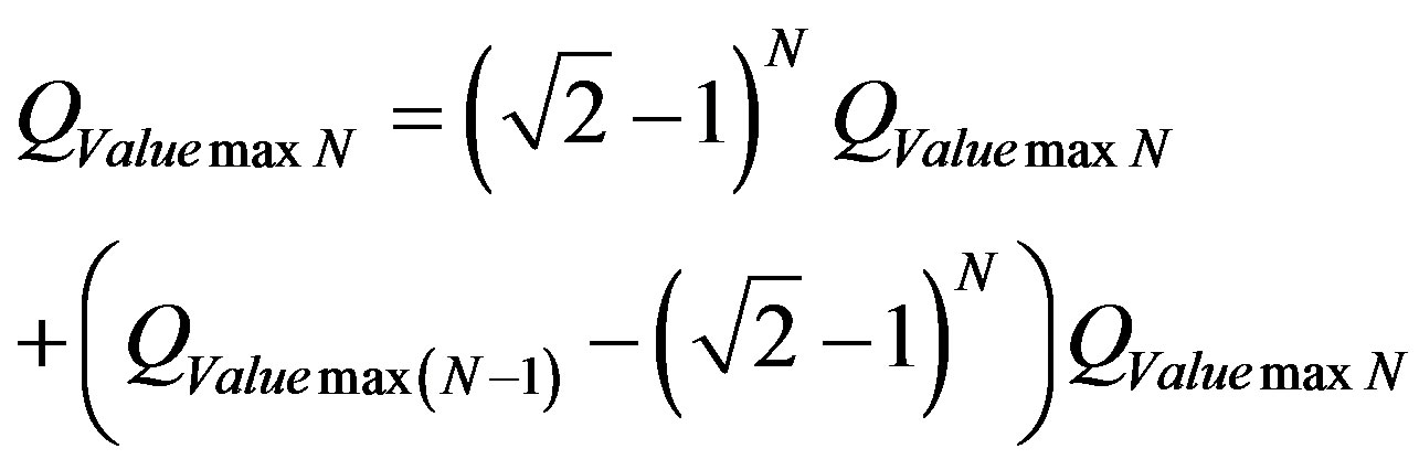 (15)
(15)
for N a natural equal or greater than 1.
For the paraquantum analysis we observe that the maximum quantity of any physical quantities in the physical world on the frequency N is composed of two quantized paraquantum fractions where:
a) one is determined on the Paraquantum logical state of Quantization ψhψ by the Paraquantum Factor of quantization to the power of N such that (hψ)N;
b) the other is determined by its complement on the frequency N.
The relation to the axis can be obtained from the values on the vertical axis of the contradiction degrees and from the values on the horizontal axis of the certainty degrees.
The analysis of the quantities in the physical environment is related to the values of Certainty Degree DC and Contradiction Degree Dct, both quantized through the Paraquantum Factor of quantization hψ (see [12,13]).
Quantization Factor of the Paraquantum Leap
Since physical systems are dynamic, the paraquantum analysis always considers the variations on the measurements performed on the Observable Variables in the physical environment which cause variations on the evidence Degrees m and l. These variations are expressed on the Lattice of the PQL and cause the propagation of the Superposed Paraquantum logical states ψsup and the occurrences of Paraquantum Leaps. So, the Superposed Paraquantum logical states ψsup are always analyzed with the features of propagation through infinitely many Paraquantum logical states of quantization ψhy defined in infinitely many Local Fundamental Lattices in the Lattice of PQL [12,14,15].
The propagation of the Superposed Paraquantum logical states ψsup through the Lattice of the PQL causes the occurrences of Paraquantum Leaps that originate effects in the form of variations on the Real Certainty Degrees— DCψR. The resulting value of this effect is added to or subtracted from the resulting value of the analysis, depending on if the considerations are being made as referring to the “arrival” or to the “departure” of the propagation. So, the value added to or subtracted from the Paraquantum Leap in the form of Real Certainty Degree— DCψR depends on the Frequency level of the Lattice or the number of times of application of the Paraquantum Factor of quantization hψ.
For the Fundamental Lattice the quantized value of the Real Certainty Degree—DCψR due to the Paraquantum Leap, which is added to or subtracted from, is computed by (11). Figure 2 shows the effect of the Paraquantum Leap in the quantization of the values when the Superposed Paraquantum logical states ψsup reach the point where the Paraquantum logical state of quantization ψhψ in the Lattice of the PQL.
We observe that in a quantitative relation the Real Certainty Degree—DCyR produced in the Paraquantum Leap on the Paraquantum logical state of quantization
ψhy is a value added to or subtracted from the total quantized value that appears at the instant of the Paraquantum Leap. So, in a relation where the quantity of the Largeness in the physical environment is related to the Degree of Contradiction Dct, the value of the Real Certainty Degree DCyR is considered as a Factor of quantization in the Paraquantum Leap as seen in (10).
For a complete equationing the total Factor Paraquantum of Quantization in the Fundamental Lattice of the PQL is expressed with the Factor related to the Paraquantum Leap, added to or subtracted from the Paraquantum Factor of quantization hψ, such as:
 (16)
(16)
We have: a)  is the Factor Paraquantum of total Quantization at the “arrival” at the Superposed Paraquantum logical state ψsup, at the equilibrium point where the Paraquantum logical state of quantization ψhψ is.
b)  is the Factor Paraquantum of total Quantization at the “departure” from the Superposed Paraquantum logical state ψsup, at the equilibrium
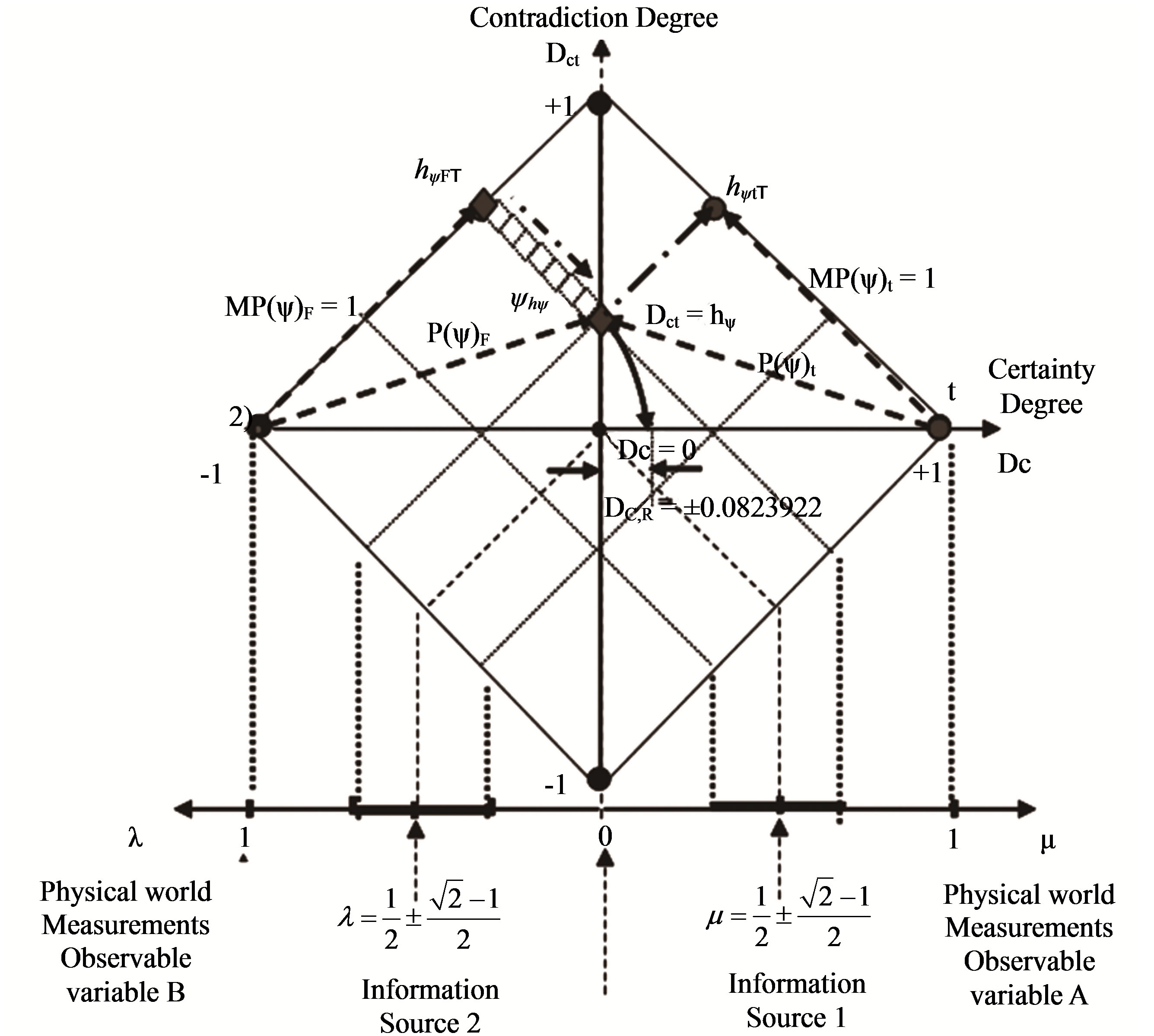
Figure 2. The Paraquantum Factor of quantization on the paraquantum logical state of quantization yhy due to Paraquantum Leap.
point where the Paraquantum logical state of quantization ψhψ is.
For Lattices of the PQL with transition frequency levels N the equation of the Factor Paraquantum of total Quantization hy is expressed as follows:
 (17)
(17)
with: a)  the Factor Paraquantum of total quantization at the “arrival” at the Superposed Paraquantum logical state ψsup, at the equilibrium point where the Paraquantum logical state of quantization ψhψN is.
b)  is the Factor Paraquantum of total quantization at the “departure” from the Superposed Paraquantum logical state ψsup, at the equilibrium point where the Paraquantum logical state of quantization ψhψN is.
With: N natural equal or greater than 1.
Using the above equation of the Paraquantum Quantization, which relates values of quantities of physical largeness to the Lattice of the PQL, can be expressed by:
 (18)
(18)
where: hψtn = N is the Factor Paraquantum of total Quantization computed by:
 (19)
(19)
We observe that hψtn=N adds the related Factor to the Paraquantum Leaps at the arrival at the propagated Paraquantum Logical states on the point N or subtracts the related Factor from the Paraquantum Leaps at the departure of the propagated Paraquantum Logical states on the point N.
3. Paraquantum Analyses in Physical Systems
Based on the above equations we present the Paraquantum Logic (PQL) as a logical solution for resolution of phenomena modeled by the laws of Physics [5,11,16]. In order to develop this study, we start its application base on assumptions made from experimental observations of the Newton laws. Doing this the PQL will allow, through the Paraquantum Logical Model [14,15], the mathematical applications to be extended to all fields of the physical science.
In the application of the model based on the Paraquantum Logics PQL in resolution of physical phenomena, we would like to emphasize the importance of the second Newton law which expresses the crucial statement about how objects move when subject to forces [12].
The idea of the second Newton law is that when a resultant of forces acts on a body, this body will receive an acceleration which is proportional to Force (F) and inversely proportional to its mass (m) [17,18]. When the law is expressed as a mathematical equation, this statement depends on a value that adjusts or defines this proportionality between the physical largenesses, such that:
 (20)
(20)
where:
a is the acceleration or the ratio through which the velocity of the body changes along time.
F is the resultant of all forces acting on the body.
M is the mass of the body.
k is a factor of adjustment of proportionality.
In order to apply the Paraquantum Logics PQL on physical systems it is important to study Newton’s laws which relate the involved physical largenesses (force, mass and acceleration) with the British System of units as well as the implications with respect to their transformations to the International System of Units (SI) [16,18]. In the British System of units those Physical largenesses considered fundamental are defined as: force, length and time. Because of that there is no freedom to choose units for force and acceleration that must be used, however, to define the unit for mass so large or so small as desired. Doing so, the value of the proportionality constant k in (38), which represents the second Newton law [16], depends on the value of the unit chosen for mass. For the unit of force when the proportionality factor k acts on the mass, where the force and the acceleration are 1 in the International System of units (SI), the equation that expresses the poundal of the British System [16-18] of units is expressed by:
 (21)
(21)
We repeat the above again but now using the corresponding values from the International System of units (SI) where the unit for force is the Newton (N). In this case, (39) can be expressed by:
 (22)
(22)
Comparisons and analogies between the Systems of units lead us to relations and values that made the proportionality factor k of (38), which represents the second Newton law, to be 1 in the International System of units (SI).
The theoretical and experimental values show that the PQL is a logic capable of creating models that can represent the physical phenomena with a good approximation of the values obtained through the equations representing the second law of Newton. So, it is possible to adapt the factors of proportionality adjustment k obtained for the Paraquantum Logical Model as follows:
and

Considering that the values of k were obtained from arbitrary measurements, whose values were adapted along the years with practical applications, the differences are low.
3.1. The Newton Gamma Factor 
This corresponds to the Paraquantum Factor of quantizetion  obtained on the equilibrium point where the Paraquantum logical state of quantization
  is located [12,13]. In the application of the Paraquantum Logical Model in broad areas of physics, the factor
 , as well as its inverse value, will be largely used to perform adjustments needed to the natural proportionality that exists between physical quantities and adjustment of unitary values between unit systems. Due to its importance, we will call this value Newton Gamma Factor and represent it by
 . Therefore, for the classical logic applied in the Paraquantum Logical Model [14,15], we have Newton Gamma Factor
 .
.
3.2. The Paraquantum Gamma Factor 
Equation (11) expresses the variation of the value of the Favorable evidence Degree µ extracted from measurements performed on Observable Variables in the physical environment, correlating to the Paraquantum Factor of quantization hψ on the lattice of the PQL.
When we consider obtaining the Favorable evidence Degree only, this equation can be written as follows:
 (23)
(23)
The condition previous to the analysis, which resulted in , can be mathematically expressed through multiplications of inverse values of the Newton Gamma Factor [12,13]. In a procedure of expansion of the lattice, keeping the inverted value of the Newton Gamma Factor in the successive applications, we can identify the Lorentz factor
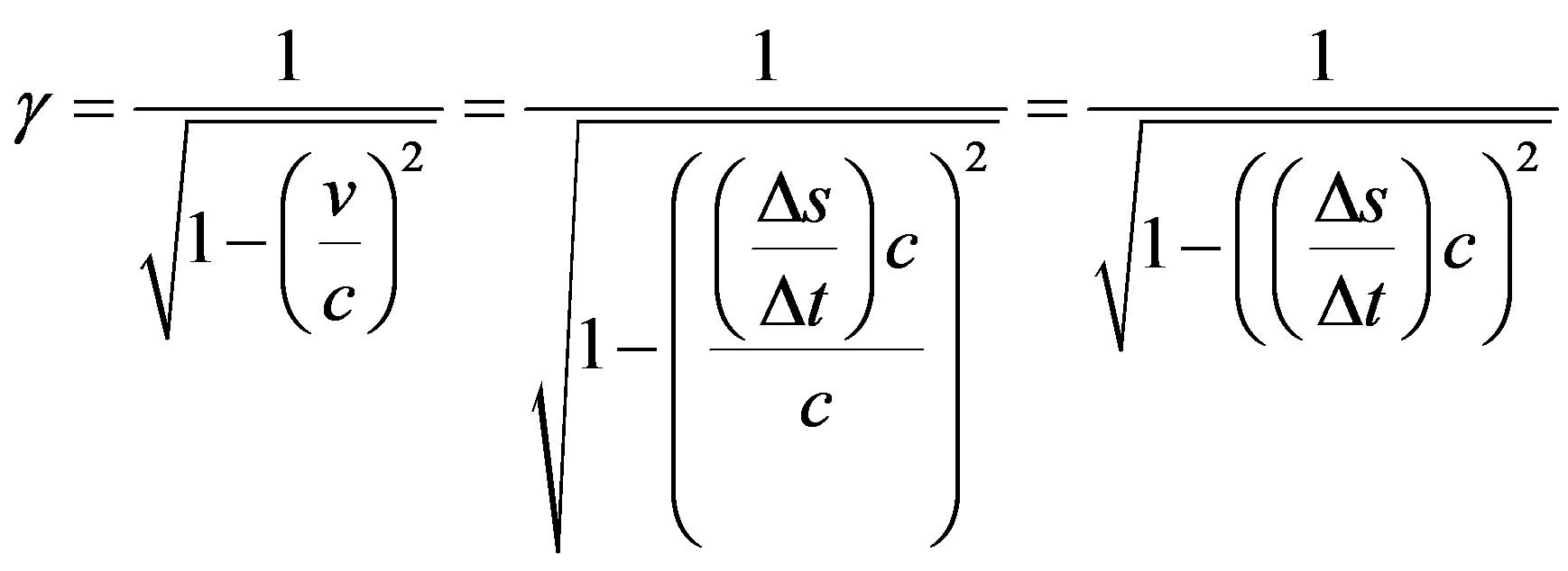
  in the infinite series of the binomial expansion. As was seen in [13] we identify a correlation value of the paraquantum logics which we call Paraquantum Gamma Factor
  such that:
 (24)
(24)
where:
 is the Newton Gamma Factor such that
 is the Lorentz Factor.
Using the Paraquantum Gamma Factor  allows the computations that correlate values of the Observable Variables to the values related to the quantization through the Paraquantum Factor of quantization hψ to be performed in any area of study of the physical science. The applications of the
  can be done from relativity theory to quantum mechanics.
3.3. The Applied Paraquantum Gamma Factor  in the Paraquantum Logical Model
The Paraquantum Logical Model is a way to study physical phenomena through the Paraquantum Logic PQL based on measurements performed on Observable Variables in the physical environment. According to what we have seen so far, the analysis between the systems of units and the adjustments with Newton’s laws which govern classical physics, produced the Newton Gamma Factor  in the paraquantum analysis [12,13].
3.4. The Variable Observable Velocity in the Primordial Lattice of PQL
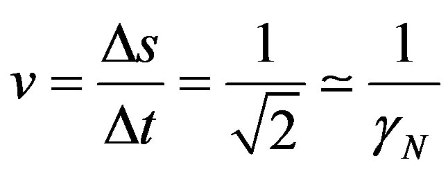
In the so called uniform linear motion (ULM) there is no acceleration and the object being studied has constant velocity v [19-21]. For this condition, according to Newton’s laws, the resulting of forces acting on the body is null. Given a displacement Δs during a measured time Δt the scalar velocity v is obtained by: .
.
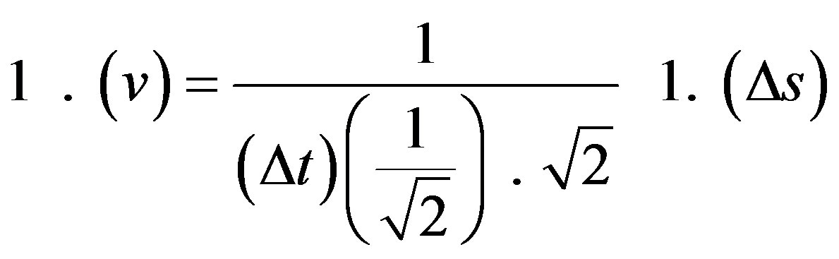
We observe that the concept of velocity or the physical state of movement in classical mechanics need two values established by measurements of two Observable Variables in the physical environment and when we consider them from the PQL viewpoint we have:
1) Observable Variable time t which appears on the equation with the measured inverse value such that:
2) Observable Variable space s which appears on the equation with the value measured such that
 In the paraquantum analysis where (24) was used, being the values of velocity v receiving repeated actions of the application of the inverse value of the Newton Gamma Factor, the velocity is related to the Primordial Lattice of the Paraquantum Gamma Factor
 , such that:
 .
.
This condition suggests values defined for a Primordial Lattice of paraquantum analysis where, at the time of obtaining de evidence Degrees from the physical environment for a fundamental unit of the Observable Variable s, there is a fundamental variation of the Observable Variable time flow t of . So, the primordial equation shows that for length 1 the velocity v of the body in relation to the speed c of the light in the vacuum is represented by the inverse value of the Newton Gamma Factor
 . However, in this condition the velocity is not 1 but:
 .
.
Considering the equation of velocity only and analyzing through the concepts of PQL, we observe that this contradiction is produced by the time t when it is seen as an Observable Variable in the physical environment.
3.5. The Measured Time t Considered as Variable Observable
Time when considered as an Observable Variable in the physical environment which is able to produce Favorable and Unfavorable evidence Degrees µ or λ, respectively, for the paraquantum analysis, but produces a measurement with features different from other fundamental largenesses, such that its values always increase and never decrease, behave as a contradiction producing factor.
Time, as expressed in the denominator of the equation of velocity is the fundamental largeness that produces in the Newton’s equations the need of the factor of proportionality adjustment and is represented in the paraquantum analysis by the Newton Gamma Factor .
.
We initially observe that for a Universe of Discourse (or Interest Interval), considered in the Paraquantum Analysis, the evidence Degree obtained from measurements of the Observable Variable time has the following properties:
1) measurements are necessarily quantized due to its fluidity.
2) its measured value always increases, never decreases, which makes it to be considered a flow of positive values.
3) in reality its value is never stable therefore can never be considered a constant.
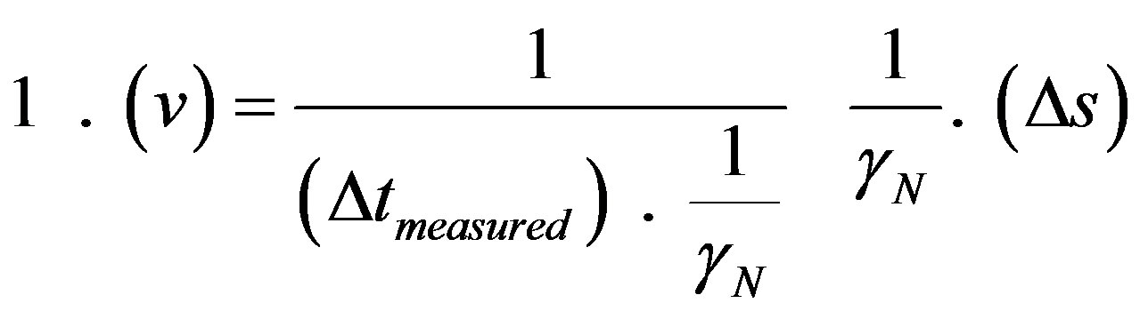
The unit of time measured, in order to be considered as maximum Favorable evidence Degree in the Primordial Lattice of the PQL, is normalized and therefore following the condition imposed to the equation of velocity has always the inverse value of the Newton Gamma Factor. So, considered in the Paraquantum Logical Model, the extraction of the evidence Degrees done through the Observable Variable time produces a quantified value of its contribution to the value of the Observable Variable velocity, which always is, in the Newtonian universe; .
.
However, since time is not unitary but shows a value of measured time similar to a flow of continuous increment, then when the Paraquantum Logical Model is effectively applied outside the Newtonian universe, the Observable Variable time receives action of the Paraquantum Gamma Factor  and produces contradiction in the analysis.
3.6. The Paraquantum Gamma Factor  and the Measured Time t
First we consider that the value of velocity v can also be represented by the measured space  divided by the measured time
 . So, the equation of Lorentz Factor
  can be expressed as follows:
In a contraction of values in the paraquantum analysis the time t is linked to the space s to receive the action of the quantization frequency η by the repeated application of the inverse value of the Newton Factor . The Primordial Lattice, with its values established in the Newtonian universe, relates time with the value of the Newton Gamma Factor
  such that:
 (25)
(25)
In the Primordial Lattice the equation of velocity is expressed with the primordial values of largenesses such that:
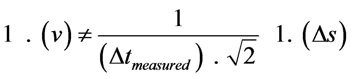
or
 (26)
(26)
We observe that in these conditions of primordial values the equality is satisfied if and only if the value of the velocity is multiplied by the Newton Gamma Factor, such that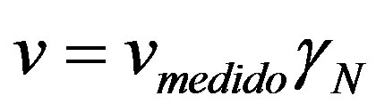 , which produces the equality expressed by:
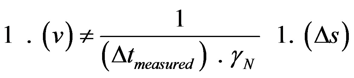
or after rewritten so that it becomes compatible with the expression of velocity of the laws of classical mechanics of the Newtonian universe:
 (27)
(27)
Considering that in the Newtonian universe the Paraquantum Gamma Factor is approximately equal to the inverse value of the Newton Gamma Factor , the equation of the velocity in the Paraquantum Logical Model can be rewritten as follows:
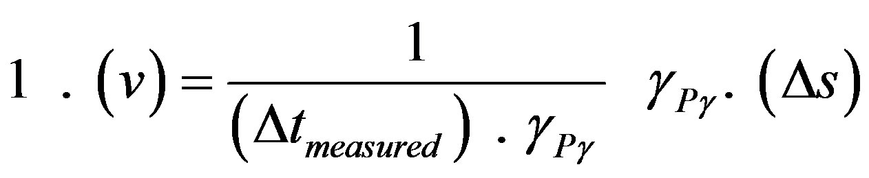
so the flow of paraquantum time is the time measured, quantified and its value is expressed by:
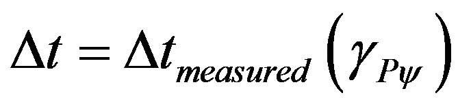 (28)
(28)
where:  = measured variation of time
 = Paraquantum Gamma Factor from (24).
The Equation (25) which deals with velocity can be written in the form where the action of the Paraquantum Gamma Factor can be visualized:
 (29)
(29)
where:  = measured variation of time.
 = measured space.
We also consider that the property of the fundamental physical largeness time has continuity of increment which means that it can never be zero.
4. The Paraquantum Physical Largenesses
Based on the considerations and equationings done with the foundations of the Paraquantum Logics PQL [12-15] we present the fundamental largenesses of Physics through the action of the quantization factors.
4.1. The Paraquantum Velocity 
The variation of the continuous increment of the value of time, whose measured value affects the value of velocity, considers that, in the Paraquantum Logical Model, its Interest Interval may change by its own action. This means that time, in its representation in the Primordial Lattice of the PQL, forces the values of space s and, as a consequence, the value of velocity v, to be multiplied by the Newton Gamma Factor  when they are measured. We can introduce a concept of paraquantum velocity such that from (29) we obtain:
 (30)
(30)
where:  = paraquantum velocity.
 = measured variation of time.
 = Paraquantum Gamma Factor.
 = measured variation of space.
The paraquantum velocity is the representation of the velocity of the body which is considered as a physical state of motion in the PQL because it is represented by a Paraquantum Logical state ψ. So, paraquantum velocity is represented through the analysis by two evidence Degrees extracted from two Observable Variables in the physical environment: time t and traveled space s. Since the longer is the time measured in equal intervals of traveled space, the lower the velocity is, then for the proposition P: “velocity is high”, the time represents the Favorable evidence Degree [3,21-23] when it is received with the resulting inverse value such that:
Favorable evidence Degree: 
Since the shorter is the space measured in equal intervals of constant time, the higher the velocity is, then for the same proposition P: “velocity is high”, the traveled space represents the Unfavorable evidence Degree when it is received with the resulting inverse value such that: Unfavorable evidence Degree: .
.
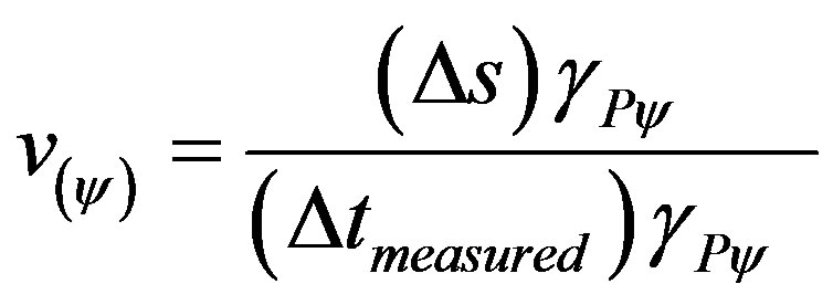
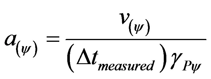
According to the foundations of the PQL, in a dynamical process the quantization of velocity will happen at the equilibrium point where the Paraquantum Logical state of quantization ψPψ is, that is, in the state that expresses the action of the Paraquantum Factor of quantizetion hψ of the P QL. Equation (30) of velocity becomes the one of the quantization of the state of velocity and is obtained by:

 (31)
(31)
where:
 = quantized value of the state of velocity or motion of the system.
 = measured time variation.
 = Paraquantum Gamma Factor.
 = measured traveled space variation.
 = Paraquantum Factor of quantization
 .
.
Writing:
 and
and 
The previous equation can be written as follows:
 (32)
(32)
where:  = measured initial space.
 = measured final space.
 = measured time at the initial traveled space.
 = measured time at the final traveled space.
In the representation that expresses the value of state of velocity in the system, all performed measurements in the physical environment related to the Observable Variables time t and space s are multiplied by the value of the Paraquantum Gamma Factor  found in (24).
In the case of motion with velocity much lower than the speed of light in the vacuum, hence in the Newtonian universe, the inverse value of the Newton Gamma Factor
 can be used due to its proximity to the value of the Paraquantum Gamma Factor
 .
.
We observe that according to (32) for any value of measurement on Observable Variables in the physical environment, there is no contradiction with the basic laws of physics in the application of the Paraquantum Gamma Factor since the values of measured time and traveled space s are captured in a sequential way and it causes the annulment of the action of the Paraquantum Gamma Factor in the physical reality. However the representation in the Lattice is only possible by the action of the Paraquantum Gamma Factor on the measurements which produces the quantization of the state of velocity through the Paraquantum Factor of quantization hψ.
4.2. The Paraquantum Acceleration 
According to classical physics [18,22,23], in the study of the uniform linear motion (ULM) the object has constant velocity and the resultant of forces acting on the body is null. For these conditions given a displacement  during time
 , the scalar velocity v is given by:
 .
.
Different from the ULM, in the uniformly varied linear motion (UVLM) the object being studied varies its velocity in a constant fashion, that is, the object has constant acceleration. So, the equation of acceleration is similar to the one of the velocity in the ULM which is:
 . In physical systems of this sort, acceleration depends on the variation of velocity v in relation to the measure time t. Since force acting on a body causes the variation of velocity as well as changes in the mass, then acceleration depends on the force F applied to the body and on its mass [20]. However Force and mass can act independently in the system with respect to the applications of force and variations of mass. In this relation between these two physical largenesses we observe that their values caused the inverse effect of varying velocity and as a consequence, the acceleration. If the mass of a body in motion increases, its velocity will decrease and if force is applied in the sense of the body’s motion, velocity will increase.
For applications in the same sense of the motion we can consider that the force causes the increase of the variation of velocity. Therefore the values of displacement, velocity and force are directly proportional to acceleration. On the other hand, the value of mass measured and the value of time measured are inversely proportional to acceleration. However, we observe that in the representation on the PQL, the variation of velocity is quantified through a Paraquantum logical state ψ produced by the analysis of measure time t and displacement s. As it was seen, time, when considered as an Observable Variable in the physical environment, has a special feature, namely, fluidity which is different from mass. However the measured time always has its value multiplied by the Paraquantum Factor of quantization and it only affects the measurements when the value of velocity variation is high. Equation (30) expresses the paraquantum velocity and can be expressed as follows:
 .
.
According to the laws of physics and using the previous equation we can obtain the paraquantum acceleration by writing the following:
 hence:
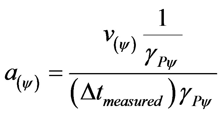
From (32) we can rewrite (31) as follows:


Taking the equation of the paraquantum acceleration to this last equality we have:
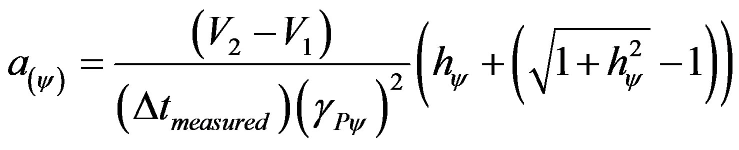 (33)
(33)
where:
 = quantized value of the state of acceleration of the system.
 = value of the final measured velocity.
 = value of the initial measured velocity.
 = measured time variation.
 = Paraquantum Gamma Factor.
 = variation of the measured traveled space.
 = Paraquantum Factor of quantization
 .
.
We observe that according to (33) for any value of measurement on the Observable Variables in the physical environment in the Newtonian universe, there will be no contradiction of the basic laws of physics in the application of the Paraquantum Gamma Factor. This happens because the Paraquantum Gamma Factor in the Newtonian universe is approximately the inverse of the Newton Gamma Factor that in the acceleration appears in its square, resulting in a denominator of the equation of approximately 0.5.
We observe that this value is very close to the part of the equation related to the Paraquantum Factor of quantization hψ which is in the numerator of the equation.
4.3. The Observable Variable Force in the Paraquantum Analysis
Being the paraquantum acceleration  as expressed in (33) and following the concepts of the Paraquantum Logics PQL, we observe that, due to the action of time on velocity, the force F that appears on (20), which represents Newton’s second law, will receive action of the Paraquantum Gamma Factor
 .
.
As it was seen for the velocity, this equation in the Primordial Lattice of the PQL will be initially written as an inequality such that: .
.
We verify that under this condition we have a natural inequality in (20) which represents Newton’s second law: this inequality happens because of inherent properties of the fundamental physical largeness time. In order to have the equality satisfied we must have the quantity of the physical largeness acceleration decreased by the action of the Paraquantum Gamma Factor . Hence, the previous inequality becomes an equality which is expressed by the following:
 where:
 which is the expression of the paraquantum acceleration. Hence, in order to obtain the value of the acceleration in the physical environment, when we have the value of the paraquantum acceleration, the equation is expressed as follows:
 (34)
(34)
where:  = value of the acceleration of the body being studied related to the physical world.
 = value of the acceleration of the body being studied related to the Paraquantum world.
 = Paraquantum Gamma Factor.
Hence, we have the equation of the paraquantum acceleration as follows:
 (35)
(35)
where:  = quantized value of the state of acceleration of the system.
 = value of the Force applied to the body being studied.
 = Paraquantum Gamma Factor.
 = mass of the body being studied.
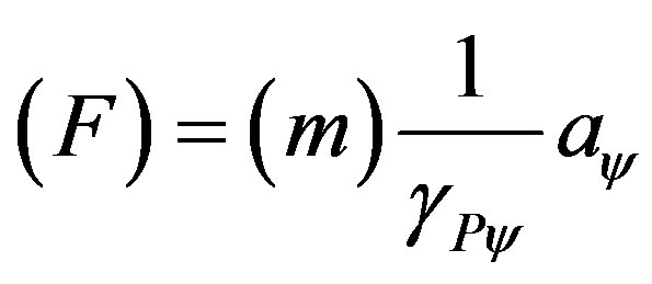
From (35), which expresses the value of paraquantum acceleration which involves force and mass, we can isolate the Force F of the paraquantum analysis such that:
Considering that the paraquantum value of Force is mass multiplied by the paraquantum acceleration, then having the value of the paraquantum Force, its value corresponding to the physical environment is given by:
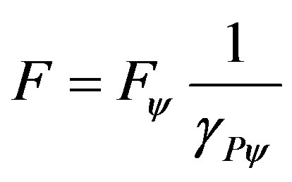 (36)
(36)
where:  = value of the acceleration of the body being studied relates to the physical world.
 = value of the acceleration of the body being studied related to the paraquantum world.
 = Paraquantum Gamma Factor.
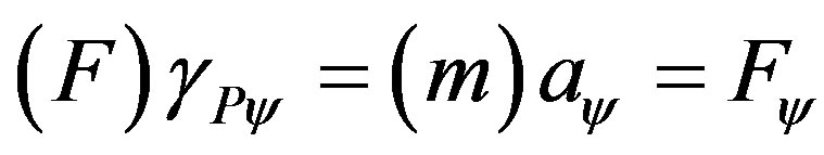
Being Force obtained by (20) such that:
Then using in this equation the expression of the Paraquantum acceleration of (33) we have:
This last equation can be rewritten in such a way the one of the Observable Variables may be represented with quantized values by the action of the Paraquantum Gamma Factor, such that:
 (37)
(37)
Equation (37) shows that in the Paraquantum Logical Model, the equation (20), which represents the second Law of Newton, can be represented with the physical largenesses quantized. Hence, for a value of Force F equal to the measured value, that is, without receiving the action of the Paraquantum Gamma Factor, we have:
a) the measured value of the variation of velocity
 is multiplied by the inverse value of the Paraquantum Gamma Factor.
b) the measured value of time variation
 is multiplied by the value of the Paraquantum Gamma Factor.
c) the value of the mass m of the body is multiplied by the inverse value of the Paraquantum Gamma Factor. Since we cannot change the features which are inherent to the fluidity of time and velocity is not directly a part of the second equation of Newton, then in (37) we still have the condition that the measured value of mass does not receive the action of the Paraquantum Gamma Factor. In this case, where we consider the value of the mass to be the measured one, the Paraquantum Gamma Factor is multiplied by the measured value of force.
4.4. The Paraquantum Average Velocity
For any sort of motion studied we consider the value of the measurement of distance of an object from its initial point is given by its average velocity (Vaverage) and the measured time t. Hence, this description can be expressed by: .
.
We observe in this equation of traveled space that its value s is obtained through the interaction of two physical largenesses where one of them is the average velocity (Vaverage) which in the paraquantum analysis is considered as an Observable Variable from which we extract an evidence Degree. However, according to the foundations of the Paraquantum Logic PQL, the average of values is an undefined situation where the evidence Degrees extracted from the measurements performed on the Observable Variables bring: Favorable evidence Degree:  and Unfavorable evidence Degree:
 . We have that the value of the average velocity is already multiplied by the value corresponding to evidence Degree of Indefinition of the Paraquantum analysis. Hence, the average velocity in the Paraquantum Logical Model has a value computed according to the laws of physics [18,20-22]. We have:
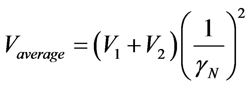
However, in the Newtonian universe, inverse value of the Newton Gamma Factor is considered, so the equation of average velocity can be expressed in a paraquantum form as follows:
 (38)
(38)
where:  = quantized value of average velocity which is equal to the value obtained by the laws of physics.
 = measured value of final velocity.
 = measured value of initial velocity.
 = Newton Gamma Factor which is
 .
.
4.5. The Observable Variable Traveled Space in the Paraquantum Analysis
Being time t considered as the other Observable Variable in the equation of space [17,21], it is also approached by the paraquantum analysis as it was studied in the previous equations, hence: .
.
The equation of traveled space can be written in a paraquantum fashion as follows:
 (39)
(39)
Since the Paraquantum Gamma Factor in the Newtonian universe is approximately equal to the inverse value of the Newton Gamma Factor such that:
then the equation of traveled space can be written with the factors in the form of values such that:
 (40)
(40)
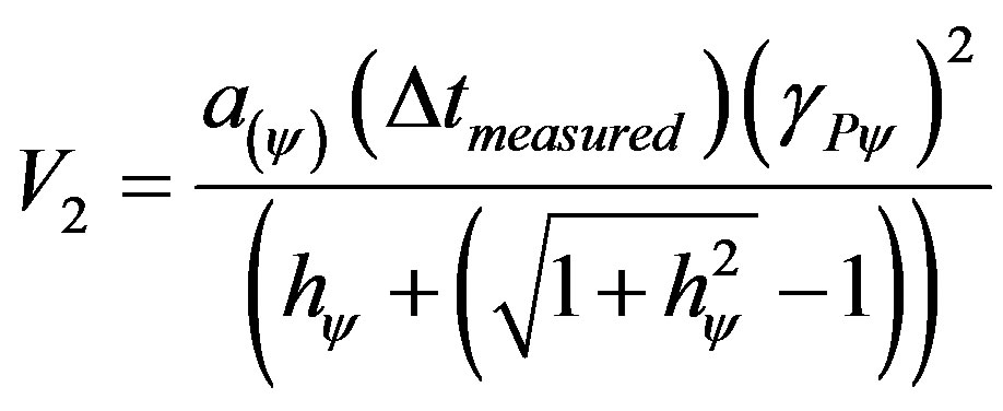
From (33) that expresses the paraquantum acceleration and using the approximation of the Paraquantum Gamma Factor as being the inverse value of the Newton Gamma Factor (40), we have:
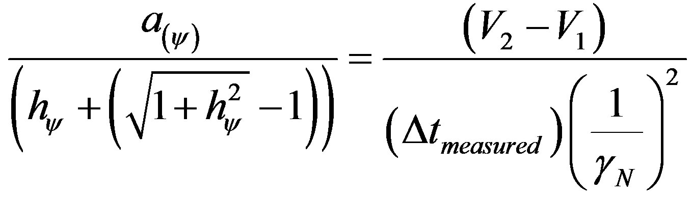
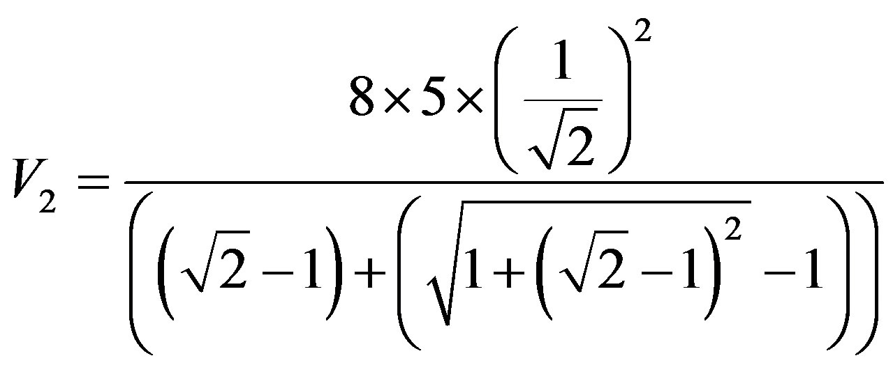
Isolating V2, we have:
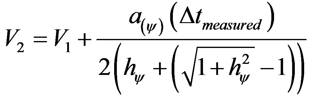 (41)
(41)
Replacing this value of V2 in (40) of traveled space ∆s, we have:
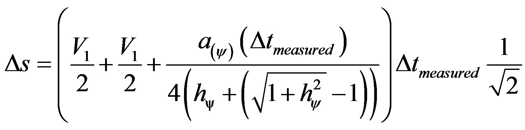
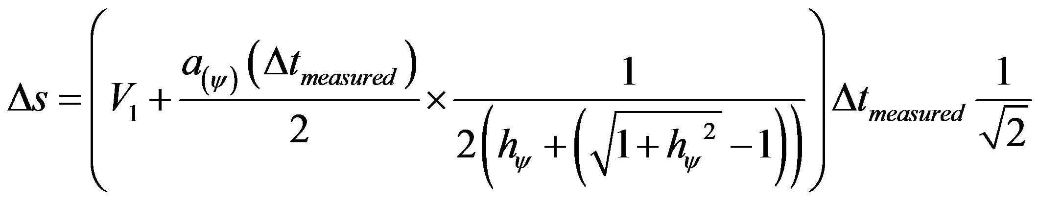
 (42)
(42)
Going back to the value of the Paraquantum Gamma Factor, the equation of space which due to the use of paraquantum largenesses expresses a paraquantum value producing it by:
 (43)
(43)
where:  = variation of space traveled obtained from paraquantum values.
 = measured value of initial velocity.
 = Paraquantum Gamma Factor.
 = measured variation of time.
 = value of acceleration of the body in study related to the paraquantum world.
 = Paraquantum Factor of quantization
 .
.
Where the equation of traveled space used in classical physics is established and the action of the Factors from the Paraquantum Logics PQL.
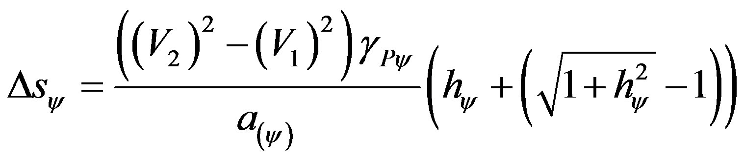
The traveled space Δs when analyzed from the paraquantum viewpoint becomes a Physical Largeness considered as an Observable Variable and the evidence Degrees are extracted from it. Hence, the space traveled which is computed by (43) is considered a paraquantum space in which, when its value is obtained, in order for it to be reported to the physical world, will have to be multiplied by the Paraquantum Gamma Factor. Hence, being ∆sψ a value of traveled space obtained by (43), the equation to report the value of traveled space to the physical world is:
 (44)
(44)
where:  = variation of measured traveled space.
 = variation of traveled space obtained through paraquantum values.
 = Paraquantum Gamma Factor.
4.6. Impulse
It is important in the paraquantum analysis to study the equation of quantity of impulse caused by force or mass which makes an object to move such that the value of the variation of velocity is represented by the paraquantum quantification: .
.
Hence, being Force represented by (37), such that:

then the Impulse will be:
 (45)
(45)
4.7. The Amount of Movement
In the analysis of Quantity of Motion the following equation is used: . Being paraquantum velocity represented by (32) such that:
Then the value of the quantity of motion is obtained by:
 (46)
(46)
5. The Energy Equations of Paraquantum Logic (PQL)
Using the equations of the physical largenesses represented in the paraquantum analysis, we present in the following the equations of energy which constitute the Paraquantum Logical Model in the analysis of Physical Systems.
5.1. Work and Kinetic Energy
We can obtain the relation between work and kinetic energy from (41) such that:
which can be written:

which replaced in (39) produces:

Still from (41) we have that:

This value replaced in (59) gives us:
which results:
 (47)
(47)
Going back to the value corresponding to the Paraquantum Gamma Factor in the Newtonian universe, we have:
 (48)
(48)
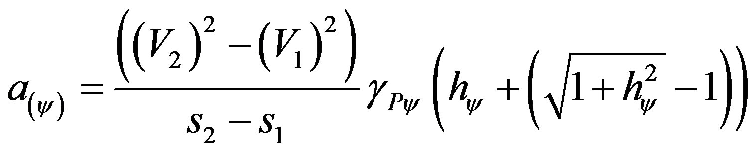
We find the equation that establishes the paraquantum acceleration when the Observable Variables which produce the evidence Degrees are values of space traveled of the square of the velocity.
 (49)
(49)
where:  = value of the acceleration of the body being studied in relation to the paraquantum world.
 = variation of the traveled space.
 = measured value of the initial velocity.
 = measured value of the final velocity.
 = Paraquantum Gamma Factor.
 = Paraquantum Factor of quantization
 .
.
Using (20), which expresses Newton’s second equation mathematically, Force can be computed by multiplying mass by the paraquantum acceleration obtained by (49) then Force can be expressed by:
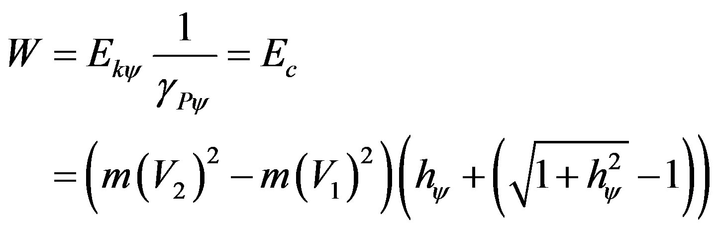
From the laws of classical physics, we know that if we multiply the value of Force by the displacement, we obtain the value of work. So, if the value for displacement is  then the paraquantum Work (Wψ) is given by the equality below:
The Paraquantum Work (Wψ ) expressed by the previous equation is identified with the total quantity of paraquantum kinetic Energy, represented on the equilibrium point of the Lattice of the PQL. This energy is composed by the quantity of kinetic energy purely quantized which is multiplied only by the Paraquantum Factor of quantization hψ, increased of Inertial Energy (or Irradiant), produced by the Paraquantum Leap at the equilibrium point. Hence, the paraquantum Work (Wψ), identified with the total kinetic Energy on the point where the Paraquantum logical State of quantization is located, is expressed in the following equality:
 (50)
(50)
Equation (50) can be written in the following fashion: pass the value of the Paraquantum Gamma Factor to the left side of the equation where its inverse value will multiply the paraquantum kinetic Energy. Hence, the value of the kinetic Energy will report to the physical world and, as a consequence, the Work performed by the body being studied. Hence, the equation of paraquantum kinetic energy, represented at the equilibrium point of the Lattice of the PQL is expressed by:
 (51)
(51)
where:  = is the quantized kinetic energy in relation to the physical environment.
 = measured value of the final velocity.
 = measured value of the initial velocity.
 = Paraquantum Gamma Factor.
 = mass of the body being studied.
 = Paraquantum Factor of quantization
 .
.
Hence, the work performed in the physical universe is identified with the quantity of quantized paraquantum kinetic Energy in relation to the physical environment such that:
 (52)
(52)
Equation (52) can be written as:

Being kinetic Energy the variation of energy of the system, from the previous equation we can obtain the paraquantum final energy such that:
 (53)
(53)
When related to the physical environment the paraquantum final kinetic energy is multiplied by the inverse value of the Paraquantum Gamma Factor, such that:
 (54)
(54)
In the same way, we can obtain the paraquantum initial energy such that:
 (55)
(55)
 = quantized initial kinetic Energy.
 = measured value of the initial velocity.
 = Paraquantum Gamma Factor.
 = mass of the body being studied.
 = Paraquantum Factor of quantization
 .
.
Similarly, the paraquantum initial energy when related to the physical environment is multiplied by the inverse value of the Paraquantum Gamma Factor such that:
 (56)
(56)
As it was seen in the concepts of the PQL, the equations of kinetic energy from (51) express the quantity of kinetic energy obtained on the point where the Paraquantum logical state ψ at the time of propagation crosses the vertical axis of contradiction degrees on the Lattice of the PQL. This is the quantized energy in which the value related to the Paraquantum Leap is included.
This value is called Inertial or Irradiant Energy (Eirr) produced by the effect or the dynamic process of the propagation of the Paraquantum Logical states. Hence, the equation of pure kinetic energy, where the Paraquantum logical state of quantization ψhψ, that is the energy on the equilibrium point where the logical states of the Lattice of the PQL propagate without the effect of the Inertial or Irradiant Energy, is computed on the initial velocity V1 by:
 (57)
(57)
When related to the physical environment, we have:
 (58)
(58)
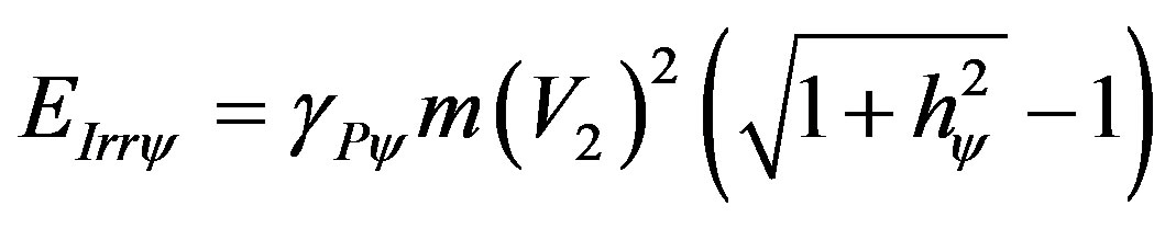
and the Inertial or Irradiant kinetic energy, produced by the Paraquantum Leap, is computed by the multiplication of the quantity related to this phenomenon whose value is represented on the horizontal axis of the Lattice of the PQL. So, the equation of Inertial or Irradiant Energy for the quantity of initial Energy is expressed by:
 (59)
(59)
When it is related to the physical environment, we have:
 (60)
(60)
Similarly, when the energy on the equilibrium point, where the logical states of the Lattice of the PQL propagate, is considered without the effect of the Inertial or Irradiant Energy, is computed on final velocity V2 by the equation:
 (61)
(61)
When related to the physical environment, we have:
 (62)
(62)
And the Inertial or Irradiant Energy produced by the Paraquantum Leap is computed by:
 (63)
(63)
When related to the physical environment, we have:
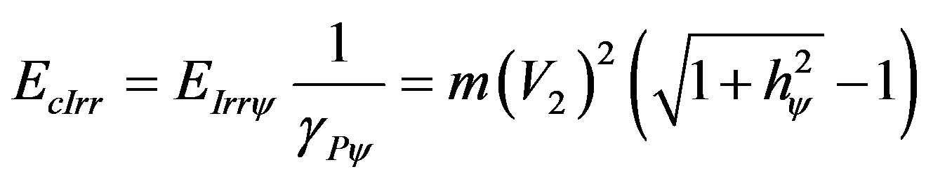 (64)
(64)
The quantity of total Energy of the Physical System in the Paraquantum Logical Model can be obtained, considering a static state, when there are no Paraquantum Leaps, hence without Inertial or Irradiant Energy or considering a dynamic state, where the effects of the Paraquantum Leaps are added in the form of Inertial or Irradiant Energy. In the equations of energy, we observe that the Paraquantum Gamma Factor multiplies the values of mass m and velocity v, which is represented by the square of its square value. This shows the action of the Paraquantum Gamma Factor  in these two Physical largenesses, which happens in any universe of physics, therefore, in any dimension of mass and velocity.
Similarly, as it was done for the space s, also the mass m, when considered in the paraquantum analysis, become a Physical Largeness treated as an Observable Variable from where we can extract evidence Degrees. So, any value of mass found through the equations of energy is considered the value of a paraquantum mass. Hence, to report its value to the physical world, we must multiply it by the Paraquantum Gamma Factor. So, being mψ a value of mass obtained through the equations that deal which energy in the paraquantum analysis, the value of mass reported to the physical world is obtained by:
 (65)
(65)
where:  = mass of the body being studied.
 = Value of mass obtained through paraquantum values.
 = Paraquantum Gamma Factor.
5.2. The Quantization of the Paraquantum Energy
The equations of energy which do not have Paraquantum Leaps (see Equations (57), (58), (61), (62)) always quantify values on the equilibrium point of the propagation of the Paraquantum Logical states. So, when the quantization of Energy through its paraquantum equations if obtained, we can compute the final quantity involved in the system in a static state. In order to obtain the total energy established in the Fundamental Lattice of the Paraquantum Logical Model without considering the effects of the Inertial or Irradiant Energy, we have to take into account the quantitative representation of these values. Hence, the quantity of total energy of the Fundamental Lattice involved in the Paraquantum Logical Model in static conditions can be obtained through (14) and it is expressed as follows:

Comparing the quantities of (14) with the quantized pure final energy obtained at the equilibrium point represented in (61) such that:
We define the total quantity of energy involved in the Paraquantum Logical Model in a static state which by comparison in the energy balance is the Total Energy of the System being that one computed in the final value of measured velocity such that:
 (66)
(66)
That when related to the physical environment, the paraquantum total energy is expressed by:
 (67)
(67)
where:  = Total Energy of the system involved in the Paraquantum Logical Model in static state.
 = Total quantized Energy involved by the Paraquantum Logical Model.
 = Final value of measured velocity.
 = Paraquantum Gamma Factor.
 = mass of the body being studied.
We observe that, since we are dealing with the total energy of the system, hence with limit values of the Lattice of the PQL, the Paraquantum Factor of quantization  does not appear in (66) and (67).
The velocity V, that in the paraquantum analysis is the final measurement of the velocity of the body related to a value of initial velocity, acts on the Paraquantum Gamma Factor through the Lorentz Factor, hence, always appear as being a fraction of the speed of light in the vacuum. For the Paraquantum Logical Model the equations which consider the velocity as Observable Variable establish V2 as a maximum velocity obtained through the measurements and that restricts the Lattice of the PQL and receives the action of factors.
In order to use an imposed limit of constant value, since the speed c of the light in the vacuum and the measurement of velocity V2 is established as a fraction of this limit and it can approach its maximum unitary value or approach its minimum null value. So, it is possible to perform a paraquantum analysis where the speed of light in the vacuum is considered constant with maximum limit 1 as follows:
Being the quantized pure final energy obtained at the equilibrium point represented in (61) such that:
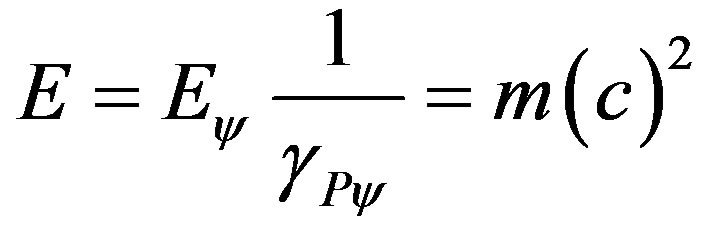
Hence, according to (20), since the Paraquantum Logical Model is normalized, then there is a complemented quantized pure energy such that:
So, the total quantity of pure Energy, that is, without Paraquantum Leaps, appears as the unity on the axis of the contradiction degrees on the Lattice of the PQL and its normalized value is computed by:
 (68)
(68)
from where the pure complemented final energy can be written taking 1 which is limited by the speed c of the light in the vacuum such that:
 (69)
(69)
where:  = complemented final quantize energy.
 = constant value of the speed of light in the vacuum imposed as maximum value.
 = measured value of velocity of the particle.
 = Paraquantum Gamma Factor.
 = mass of the body being studied.
From (69) we can write the paraquantum/relativistic equation such that:
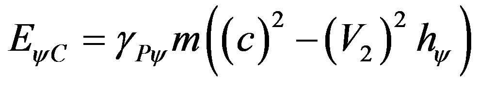 (70)
(70)
So, taking the measurements of V2 as a reference, in the Newtonian universe, when we compare values of V2 with the speed of light, the value of the constant c predominates. So, the Fundamental Lattice of the PQL is bounded by the velocity c of light such that now it is possible to obtain the paraquantum pure total energy taking into account the maximum limit, considered as the speed of light in the vacuum in the approximate equation such that:

that when related to the physical environment is expressed by:
 (71)
(71)
The Paraquantum equations of physical largenesses, such as quantity of Energy Q or relativistic momentum P as well as other largenesses belonging to the several areas of physics can be written from the concepts here presented.
6. Selected Examples of Application of Paraquantum Equations
For a detailed study of the Paraquantum Logical Model presented by the equations studied here, we present some numerical examples [17-21] with applications of the equations obtained by the Paraquantum Logical Model.
We also compare our examples with the traditional resolutions through the physical laws [17,20,23].
6.1. Example 1
VII.1a. Let us consider that a body starts its motion from rest with a constant acceleration of 8 m/s2 and we want to compute its instant velocity v after 5 s.
For this resolution we observe that there are velocity v and constant acceleration a of the body during the analysis time. Using the laws of classical mechanics, the equation for the resolution is: .
.
So,
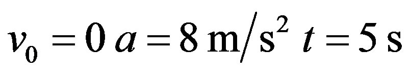 we have:

and gives us the instant velocity .
.
Using the Paraquantum Logical Model in this problem, initially we have to consider that in the physical world the observable variable time provides us with the measured value such that: . Equation (33), which relates acceleration with velocity and time, provides us with the conditions to obtain the paraquantum velocity:

So, for V1 = 0, we have:
Since we consider in the Newtonian universe
 and
and , we replace the value in the equation:

which results:

VI.1.b. Let us consider now that in the same above question, we want to compute the average velocity in the first 5s of its motion. For the resolution we use the laws of classical mechanics where the equation for this problem that computes the average velocity of the body is:
Since  and
and  the application of the equation results:

According to what was studied of the fundamental concepts of the Paraquantum Logics PQL we know that the representation of the results through averages destroys the information that is inserted in the contradiction. Hence, for a resolution where the Paraquantum Logical Model is used, we observe that the value corresponding to the average between two measurements of the same largeness is not allowed in the analysis. The exception is that the measurement might be used as evidence Degree of an analysis that involves other measurements. However, a representation of average velocity is identified when the value of the physical largeness is quantified through the inverse value of the Newton Gamma Factor for an application frequency N = 2. In this case the sum of the values has its value divided by half. In order to find the average velocity of the example question, we use (38) where:
 .
.
Since the initial velocity is null  and the final velocity is
 , then using (38) we have:
 →
→
which results:
VI.1.c. We consider the same question and now we want to know the traveled space after 5 s. In order to solve this problem we use the laws of classical mechanics which related traveled space with other physical Largenesses such that:

Therefore:
which results in traveled space: .
.
Traveled space can be found by the classical equation which expresses the value of the average velocity.
We know that:
 .
.
And we get the value for space:

The resolution in the Paraquantum Logical Model can be done through the application of (43) such that the paraquantum traveled space is obtained by:

Being:  with
with  e
e we have:
which results the paraquantum traveled space computed in the Paraquantum Logical Model of:
 .
.
This value of traveled space is called paraquantum because, besides being computed from paraquantum largenesses, its value contributes that, during analysis, the Paraquantum logical state of quantization ψhψ is located at the equilibrium point of the Lattice. So, in order for this value to be represented in the physical world, it must be multiplied by the inverse value of the Paraquantum Gamma Factor according to (44). In the Newtonian universe, the inverse value of the Paraquantum Gamma Factor is approximately the Newton Gamma Factor such that:
 →
→
Resulting: 
Similarly, the resolution in the Paraquantum Logical Model can be done also through the application of (48) such that:
Being: , with
  and
and  we have:

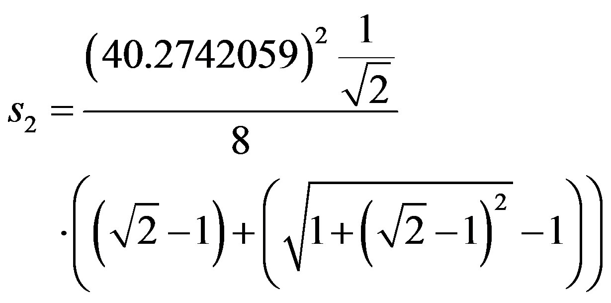
which results: .
.
Similarly, since it is a paraquantum value, in order to report it to the physical world, it will be multiplied by the inverse value of the Paraquantum Gamma Factor, which, in the Newtonian universe, is approximately equal to the inverse value of the Newton Gamma Factor such that:
Resulting: 
6.2. Example 2
VI.2a. A car whose weight is 1000 Kgf is moving on a horizontal road with a velocity of 90 Km/h. After the brake system was activated the car stopped after traveling 70 meters. Compute the brake acceleration of the car.
Resolution: The initial velocity of the car at the instant t0 of the braking is:
The variation of traveled space from the instant t0 until the car stopped at instant t1 is: .
.
Using the equation of the classical physics which involves velocity and acceleration, we have:
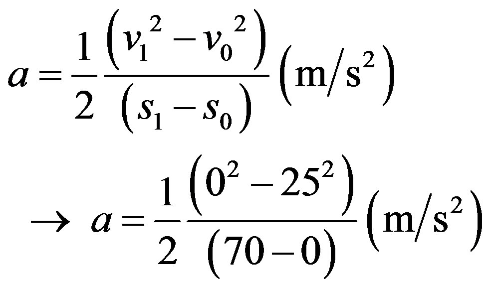
For the resolution in the Paraquantum Logical Model we first compute the paraquantum acceleration through (49) such that:
With:  and
and , then replacing:
Results in a paraquantum acceleration:

According to (34) this value of acceleration obtained, when reported to the physical world, it is multiplied by the inverse value of the Paraquantum Gamma Factor such that:

Resulting:

VI.2.b. Compute the retarding force of the brakes for this problem.
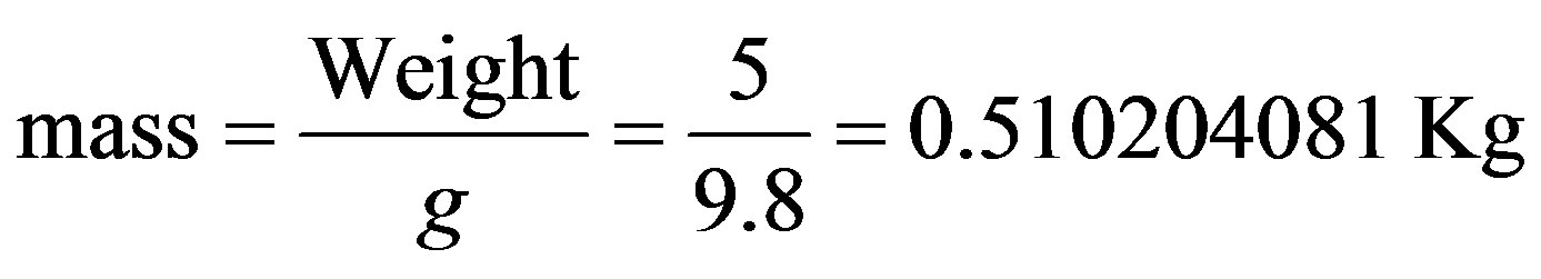
The car’s weight is: P = 1000 Kgf, so we compute the mass:

By Newton’s second law we have in the International System (SI) the force computed by:

or 
Resulting: 
According to (55): , so the value of the paraquantum Force is obtained by multiplying the mass of the body the value of the paraquantum acceleration: Being:
And 

Results the paraquantum retarding force:
According to (36) this value of Force when reported to the physical world is multiplied by the inverse value of the Paraquantum Gamma Factor that, in the Newtonian universe is approximately equal to the Newton Gamma Factor. So, the Force is obtained by:
and results the retarding Force:
6.3. Example 3
VI.3a. An object with weight 5 Kgf falls down vertically from a height h1 of 3m. Compute the velocity at the moment that the object reaches the ground.
Resolution:
The work performed on the object by the resulting force during this displacement is obtained by:
From the work-energy theorem the result is equal to the variation of kinetic energy such that:
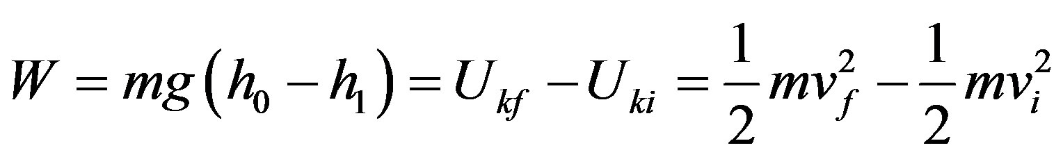
Being:  then:
then:
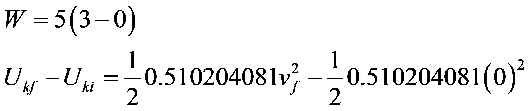

Resulting the speed:

In order to compute through the Paraquantum Logical Model we apply (52) where we consider Work performed in the physical world and compared to the total kinetic Energy at the equilibrium point multiplied by the inverse value of the Paraquantum Gamma Factor such that:
Being:  and since Work is defined by:
 , so from (52), we have:
 Resulting in the following velocity value →
 .
.
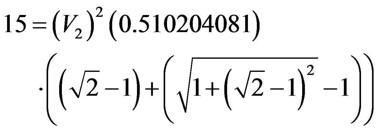
VI.3b. For the same previous condition, compute the kinetic Energy of the body.
Being:  and
and
 , then:
 ,
, 
Results: 
Being:  and
and
 then, from (72):

Compute the Paraquantum final energy such that:
And results the paraquantum Kinetic Energy:

As it was done for other largenesses, the value of energy reported to the physical world is multiplied by the inverse value of the Paraquantum Gamma Factor such that:

Resulting the final kinetic Energy:
6.4. Example 4
VI.4a. It is known that the electron-volt (eV) is the energy acquired by an electron when submitted to an electric Potential Difference of 1 volt.
The relation between the electron-volt and the energy unit Joule used in the International System of units is given by:

Considering that the mass of an electron is  what is the energy at rest of the electron in Joules and in electron-volts?
Resolution:
Using the relativistic equations, we consider the Lorentz Factor as being 1 and we have that the energy at rest of the electron in Joules is computed by:

 and establishing the relation:

So:
Since it was decided that the Paraquantum Gamma Factor is 1, which implies that the velocity V2 is null, the results will be the ones for the paraquantum analysis and for the relativistic equations.
We observe that in (70) we find the energy at rest of the electron as being the pure total energy that appears complemented, since the Paraquantum Leaps are considered:
 .
.
In order to compute the energy at rest of the electron through the Paraquantum Logical Model, we follow a procedure similar to the relativity theory and we observe that the energy at rest of the electron is considered when the Lorentz Factor is 1.
This condition implies by the equation of the Lorentz Factor that the velocity V2 is zero and through (24) we observe that this condition also implies in a Paraquantum Gamma Factor:
 .
.
We can write the paraquantum kinetic energy equation as follows:
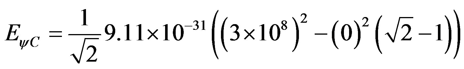
Which results in a paraquantum energy at rest of:

As it was done for other largenesses, the value of energy reported to the physical world is multiplied by the inverse value of the Paraquantum Gamma Factor such that:
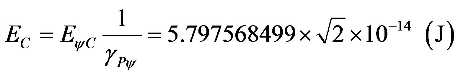
Which results in the Energy at rest of the electron:

Which in electron-volts results:


6.5. Example 5
VI.5a. If in the relativistic rest condition of the electron, which in the paraquantum analysis has the meaning of complemented energy, the condition of Paraquantum Gamma Factor  were considered, compute the velocity of the electron and its complemented energy. In this special condition where the Paraquantum Gamma Factor is 1, there is a value for the Lorentz Factor, which is obtained from (24) such that:
  when made equal to 1 results:
 . Since the Newton Gamma Factor is constant in any universe and is
 , we have:
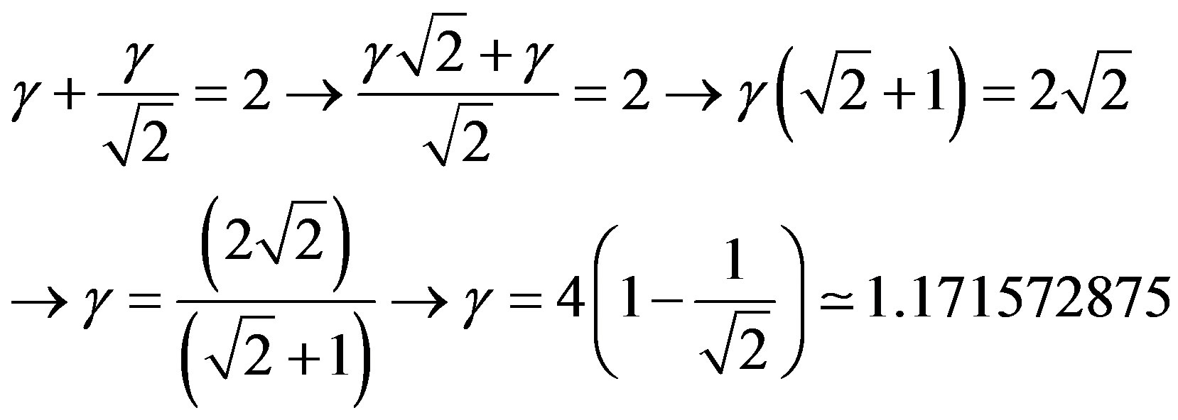
Hence the imposition of the Paraquantum Gamma Factor to be 1 propose the existence of a paraquantum velocity presumed to be of the electron for this condition where its value is computed through the Lorentz Factor from where we isolate velocity: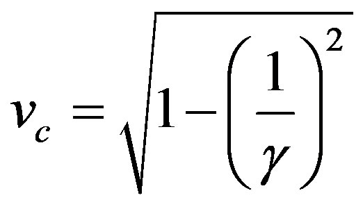 . Therefore:
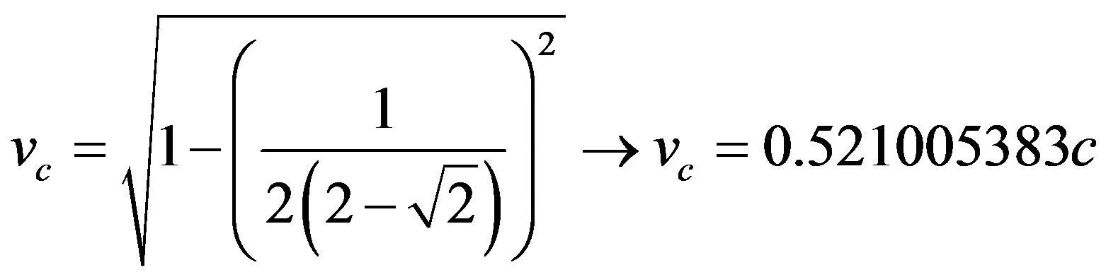
So, with values on (70) related to paraquantum kinetic energy, we have:
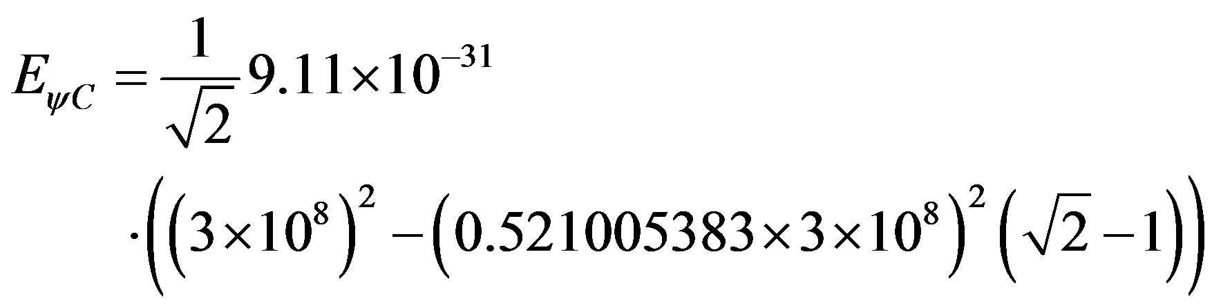

Which results in a paraquantum energy at rest of:
According to what was done for the other largenesses, the value of energy reported to the physical world is multiplied by the inverse value of the Paraquantum Gamma Factor such that:
Results in the Energy at rest of the electron:
Which in electron-volt results:
7. Conclusions
In this paper we presented the main basic concepts of the Paraquantum Logics PQL as well as the action of its equations in analysis of real physical systems. Examples of application and use of the paraquantum equations in real systems showed the capability of analysis of these concepts and foundations proving that they are able of being applied in several fields of study in Physics. In the equationing of physical largenesses through paraquantum logics and in the proofs presented in these studies we present the two most important factors of the paraquantum analysis: the Paraquantum Gamma Factor  and the Paraquantum Factor of quantization
 . We presented equations involving these two factors, whose properties allow the expansion and the contraction of the Lattice of the PQL which represents the paraquantum universe. So, through the factors it is possible to link the physical universe, founded on the Newton’s laws, with the paraquantum universe, which through its equations, can expand or contract, allowing conditions for analysis of natural phenomena in extreme limits.
We presented numerical examples of application where the results prove the existence of the correlation between the Paraquantum Gamma Factor , which operates on the measurements performed for the extraction of the evidence Degrees in the physical world, with the Paraquantum Factor of quantization
  which due to its action on the quantification of energies is identified with the Planck constant h. This correlation between the two worlds through the link produced by the two factors, allows that the Paraquantum Logical Model is capable of analyzing efficiently and in a quantitative fashion physical largenesses in any area of study of Physics.
REFERENCES
- D. Krause and O. Bueno, “Scientific Theories, Models, and the Semantic Approach,” Principia, NEL—Epistemology and Logic Research Group, Federal University of Santa Catarina (UFSC), Brazil, 2007, pp. 187-201.
- N. C. A. Da Costa, V. S. Subrahmanian and C. Vago, Mathematical Logic Quarterly, Vol. 37, 1991, pp. 139-148. doi:10.1002/malq.19910370903
- J. I. Da Silva Fiho, G. Lambert-Torres and J. M. Abe, “Uncertainty Treatment Using Paraconsistent Logic: Introducing Paraconsistent Artificial Neural Networks,” IOS Press, Amsterdam, 2010, p. 328.
- J. M. Abe and J. I. Da Silva Filho, “Inconsistency and Electronic Circuits,” In: E. Alpaydin, Ed., Proceedings of EIS’98 International ICSC Symposium on Engineering of Intelligent Systems, Vol. 3, Artificial Intelligence, ICSC Academic Press, Rochester, 1998, pp. 191-197.
- N. C. A. Da Costa, Notre Dame Journal of Formal Logic, Vol. 15, 1974, pp. 497-510. doi:10.1305/ndjfl/1093891487
- N. C. A. Da Costa and D. Marconi, The Journal of NonClassical Logic, Vol. 6, 1989, pp. 5-32.
- H. Reichenbach, “Philosophic Foundations of Quantum Mechanics,” University of California Press, Berkeley, 1944.
- J. A. Wheeler and H. Z. Wojciech, “Quantum Theory and Measurement,” Princeton University Press, Princeton, 1983.
- J. I. Da Silva Filho and A. Rocco, “Power systems Outage possibilities analysis by Paraconsistent Logic,” Power and Energy Society General Meeting on Conversion and Delivery of Electrical Energy in the 21st Century, Pittsburgh, 20-24 July 2008, pp. 1-6.
- H. A. Blair and V. S. Subrahmanian, “Paraconsistent Logic Programming,” 7th Conference on Foundations of Software Technology and Theoretical Computer Science, Pune, 17-19 December 1987. doi:10.1007/3-540-18625-5_59
- N. C. A. da Costa, D. Krause and O. Bueno, “Paraconsistent Logics and Paraconsistency,” In: D. Jacquette, D. M. Gabbay, P. Thagard and J. Woods, Eds., Philosophy of Logic, Elsevier, Series Handbook of the Philosophy of Science, Vol. 5, 2006, pp. 655-781.
- J. I. Da Silva Filho, Journal of Modern Physics, Vol. 2, 2011, pp. 1397-1409. doi:10.4236/jmp.2011.211172
- J. I. Da Silva Filho, Journal of Modern Physics, Vol. 2, 2011, pp. 1455-1469. doi:10.4236/jmp.2011.212180
- J. I. Da Silva Filho, Journal of Modern Physics, Vol. 3, 2012, pp. 233-254. doi:10.4236/jmp.2012.33033
- J. I. Da Silva Filho, Journal of Modern Physics, Vol. 3, 2012, pp. 312-333. doi:10.4236/jmp.2012.34044
- P. A Tipler,. and. A. Llewellyn “Modern Physics,” 5th Edition, W. H. Freeman and Company, 978-0-7167-7550- 8, 2007.
- J. P. Mckelvey and H. Grotch, “Physics for Science and Engineering,” Harper and Row, Publisher, Inc., New York/ London, 1978, 426 pages.
- P. A Tipler, “Physics,” Worth Publishers, Inc., New York, 1976.
- P. A Tipler and G. M. Tosca “Physics for Scientists,” 6th Edition, W. H. Freeman and Company, New York, 2007.
- M. Ference Jr., H. B. Lemon and R. J. Stephenson, “Analytical Experimental Physics,” 2nd Edition, University of Chicago Press, Chicago, 1956.
- F. Gross, “Relativistic Quantum Mechanics and Field Theory,” John Wiley & Sons, Inc., Hoboken, 1993, p. 97.
- D. Kleppner and R. K. Binding, “An Introduction to Mechanics,” Mcgraw-Hill, Columbus, 1973.
- J. Bernstein, P. M. Fishbane and S. G. Gasiorowicz, “Modern Physics,” Prentice-Hall, New York, 2000.