Applied Mathematics
Vol.5 No.8(2014), Article ID:45516,12 pages DOI:10.4236/am.2014.58104
Uncertainty in a Measurement of Density Dependence on Population Fluctuations
Hiro-Sato Niwa
National Research Institute of Fisheries Science, Yokohama, Japan
Email: Hiro.S.Niwa@affrc.go.jp
Copyright © 2014 by author and Scientific Research Publishing Inc.
This work is licensed under the Creative Commons Attribution International License (CC BY).
http://creativecommons.org/licenses/by/4.0/


Received 25 February 2014; revised 25 March 2014; accepted 1 April 2014
ABSTRACT
This article discusses the question of how elasticity of the system is intertwined with external stochastic disturbances. The speed at which a displaced system returns to its equilibrium is a measure of density dependence in population dynamics. Population dynamics in random environments, linearized around the equilibrium point, can be represented by a Langevin equation, where populations fluctuate under locally stable (not periodic or chaotic) dynamics. I consider a Langevin model in discrete time, driven by time-correlated random forces, and examine uncertainty in locating the population equilibrium. There exists a time scale such that for times shorter than this scale the dynamics can be approximately described by a random walk; it is difficult to know whether the system is heading toward the equilibrium point. Density dependence is a concept that emerges from a proper coarse-graining procedure applied for time-series analysis of population data. The analysis is illustrated using time-series data from fisheries in the North Atlantic, where fish populations are buffeted by stochastic harvesting in a random environment.
Keywords:Population Dynamics, Stochastic Difference Equation, Noise Color, Coarse Graining, Ecological Time-Series

1. Introduction
The nature of the negative feedback relationship between population growth rate and abundance is at the heart of population ecology. That said, statistical detection of density dependence using ecological time-series can be problematic. When plotting data on the form of the dependence of population growth rate on abundance, ecologists have been confounded by considerable noise around each relationship [1] . Hassell et al. [2] first pointed out that density-dependent effects are more marked in populations monitored longer. Brook and Bradshaw [3] , examining the time-series data of 1198 species, demonstrated a relationship between length of monitoring and increasing evidence for density dependence. However, the duration of a time-series necessary to distinguish a regulated population trajectory from a random walk is still uncertain [4] [5] .
A relevant serious concern is the issue of noise color: how does the presence of serial correlation in the external stochastic forcing affect the density dependence in a population? Solow [6] demonstrated that, when a statistical test of density dependence being applied to time series generated by a correlated random walk, the proportion of simulations for which the null hypothesis (random walk model) was rejected was far greater than the significance level for negatively correlated variations (blue noise), and much smaller for positive autocorrelation (red noise). The effects of colored environmental variations on modulating the population elasticity have not been analyzed quantitatively.
This article investigates the analysis of ecological time-series when the aim is to measure density dependence in the demographic processes. The equilibration time [7] [8] of the stochastic process is an informative summary measure of the dynamics of a system, describing a key property of population dynamics [9] [10] . The reciprocal of equilibration time approximates the speed of return to the equilibrium point, i.e. the elasticity (expressing the same concept as the term “density dependence” or “negative feedback” in population dynamics). The objective of this article is to explore the relation between the length of monitoring and the uncertainty in measuring density dependence: how long of a time-series is required to be able to discriminate between density-dependent signal and external noise in the ecological systems? I start with a linear approximation of a discrete-time population dynamics model [11] -[16] , where populations fluctuate slowly under locally stable (not periodic or chaotic) dynamics with low to moderate elasticity [17] . The analysis is illustrated using time-series of annual census of exploited fish populations in the North Atlantic.
2. Population Dynamics
2.1. Discrete-Time Langevin Equation
The population renewal process  of marine exploited fishes, responding to stochastic harvesting in a stochastic environment, is described by a discrete-time dynamics
 (1)
(1)
with a growth-survival factor ![]() dependent on spawner abundances S, i.e. the escapement of adults from the harvest Y. The population biomass grows as a result of, not only growth of the surviving escapees in body weight, but also of recruitment of offspring
dependent on spawner abundances S, i.e. the escapement of adults from the harvest Y. The population biomass grows as a result of, not only growth of the surviving escapees in body weight, but also of recruitment of offspring![]() . During year t an amount
. During year t an amount  is harvested with a fraction
 to the harvestable adult population, where
  denotes the fishing mortality.
All density dependence is assumed to be exerted by the adult population S [16] . It is a common observation that recruitment is unrelated to egg numbers over a wide range of spawner abundances [18] -[20] . Stochasticity enters the population dynamics in two ways, both as environmental variation mirrored by recruitment variability and as variation in the fishing mortality. Recruitment is presumed to track autocorrelated fluctuations in environmental variables. Fishers would expect this year to get as much catch as last year; there would also be some kind of inertia of fisheries management. There exist memory effects: adjacent values in the time-series of recruitment and catches-to-escapement ratio are correlated [21] .
In a stationary state (with equilibrium quantities denoted by the “ ” subscript), Equation (1), log-transformed, gives
  with the stationary fishing mortality
 , where
  is the stationary ratio of each year’s recruitment to the harvestable adult population. The relative deviations from equilibrium point are denoted as
 ,
,  , and
, and . Natural and human-caused forces
  are considered as external disturbances. On the assumption that we are free to change
 ![]() and F independently of S around the equilibrium point, linearizing (log-transformed) Equation (1) yields a difference equation
and F independently of S around the equilibrium point, linearizing (log-transformed) Equation (1) yields a difference equation
 (2)
(2)
with constant coefficient  evaluated at equilibrium. The coefficient
  measures the (linear) elasticity of the system with respect to change in population size at equilibrium. The successive difference
  approximates the annual rate of increase of a population. For generating temporally structured noise,
![]() ’s are both assumed to be described as a first-order autoregressive, AR(1), process with serial correlation coefficients
’s are both assumed to be described as a first-order autoregressive, AR(1), process with serial correlation coefficients  and driven by mean-zero iid shocks. The linear stochastic difference Equation (2) is a discrete-time analogue of the Langevin equation driven by AR(1) processes. The autoregression coefficients are calculated by using the von Neumann’s ratio [22] [23] , the ratio of the mean square successive difference
  to the variance
  for AR(1) variable
![]() , that is,
, that is, . Equation (2) is iterated to give the
  -year difference of population size
 (3)
(3)
with .
.
2.2. Equilibration Time
The population process with multiple decay-rate constants  is considered to calculate the asymptotic decay-time constant
 , i.e. the total equilibration time; the approach follows Roughgarden [11] . Let
 . Taking the mean squares over Equations (2) and (3) mediates the following two relations, respectively,
 (4)
(4)
with the ratio of the mean square successive difference  to the variance
  in population size
 , and
, and
 (5)
(5)
with the autocorrelation function of series  at lag
  years
years
 (6)
(6)
where the correction (the second term on the right-hand-side) is due to memory effects of external perturbations. From the recursion,  , a corollary to Equation (5) is obtained:
 (7)
(7)
Equations (4) and (7) yield the quadratic equation for the elasticity 
 (8)
(8)
Thus, the (linear) response of a system to external perturbations is expressed in terms of fluctuation properties of the system in equilibrium. The elasticity and the variance of population fluctuations cannot be independent, but they are related to each other in the equilibrium system [24] .
The average relaxation time of population fluctuations defines the total equilibration time  as follows [24]
 (9)
(9)
After the time  memory of the initial conditions is lost: the deviation from the equilibrium is expected to decay away in an exponential fashion with a time constant given by the equilibration time
 . The total elasticity with respect to change in population size measures the strength D of total density dependence [10] [16] :

i.e. the expectation of change in population size given  is equal to 100 × D percent negative feedback. Since the total density dependence is the asymptotic multiplicative growth rate of population per year,
  reads the asymptotic decay-rate constant. Smaller values of D indicate that systems return to equilibrium slower. Since the exponential-decay time is the inverse of the decay-rate constant, the total density dependence reads

Therefore, the density dependence D and the variance of population fluctuations are related to each other through the relation  with Equation (5).
2.3. Indeterminacy in Population Dynamics
Equation (2) with (8) yields

(where each term is standardized), implying that, if a population is governed by slowly damped dynamics , external noises mask signals for evidence of deterministic behavior of the system. Unless the population exhibits damped-oscillator dynamics (i.e. over-compensation,
 ), the relationship between
  and
and  is characterized by large variance in growth rate; most of the changes in population size occur in a density-independent manner. If a perturbation brings the system away from the equilibrium point such that
 , then the deterministic signal becomes visible over the noise; using Equations (4) and (5) this inequality reduces to

with

When one performs some observations for L years, the uncertainty in locating the population equilibrium,
 , i.e. the standard deviation of the sample mean
 , propagates into the density dependence. The variance of
  is written as [13] [16] ,
 . Making use of the explicit form for the autocorrelation function (6) yields

with

By virtue of Equation (9), a time-equilibrium uncertainty relation is obtained:
 (10)
(10)
where  denotes a remainder term of order
  given by
 . Thus, Lc provides another measure of the time scale of population dynamics, and reads
  for
for ![]() with large valued
with large valued
 . Any observation over a short duration is associated with large indeterminacy. The supposed population equilibrium
  (chosen as the sample mean) and the length of time-series data are complementary: the uncertainty of population equilibrium is decreased by increasing the duration of observation. Lc is designated the complementary time. It is worth pointing out that the complementary time is always positive for
 , while the equilibration time can acquire either non-negative real number or complex number.
2.4. Coarse Graining
Let CL be the degree of certainty, with which the supposed equilibrium lies within the bounds  :
:

for normally distributed population fluctuations (with the true (population) standard deviation ). This is equivalent to
 . Let
. Let  be the sample mean, taken under the condition that n is larger (smaller) than the supposed equilibrium point, where
  is the number of observations
  in the time-series. The negative relationship of conditional sample mean of growth rate,
  , versus
  is expected to be visible with a probability CL. The larger the probability CL, the more accurately the density dependence D is measured from the population time-series.
In order to calculate the probability CL, I analyze the time-series at different resolutions by constructing a coarse-grained time-series. Let  and
and  be the ceil and the floor functions. The coarse-grained time-series is built by taking the average inside a non-overlapping moving window with
  data points,

The coarse-grained time-series are considered to be serially independent. Accordingly, the uncertainty of population equilibrium (the standard deviation of the mean) is calculated to be

and the statistic
 (11)
(11)
has a standard Gaussian distribution. In reality, we only have the sample standard deviation. So, replacing  in Equation (11) by the square root of the sample variance,
  , yields a statistic which has Student’s t-distribution with
  degrees of freedom (d.f.); we can use the Student’s t-statistic to see how good the estimate of equilibrium population size. The value of CL, i.e. the integral of Student’s t-PDF between
 , quantifies the ability to infer density dependence from a given (long) observation time-series, and
  is the two-tailed
  percentage point of Student’s t-distribution with
 . Accordingly, the following holds
 (12)
(12)
(precisely the left-hand-side involves the remainder term of order ). After L years’ observation the negative relationship is visible with a probability of CL. Equation (12) with
  and
and  yields
 , implying that, when the observation series is longer than Lc years, the negative relationship is visible with a probability of 78.4% or more. When monitoring an equilibrium population (in the dynamic balance) for L years, the probability of the true equilibrium lying outside the bounds
  reads
reads ; the sample mean growth rate
  will then be observed, even when
 . The density dependence will be invisible with a probability of
 , that is, it has a tendency to overshoot and to leave the center point
  (i.e. sample average).
2.5. North Atlantic Fisheries
Empirical analysis [21] [25] suggests that population time-series from the North Atlantic fisheries are asymptotically stationary. The notion of asymptotic stationarity means that the probability density function of the variable monitored over a wide time interval exists and it is uniquely defined. The logarithmic changes in annual spawner abundance,  , are Gaussian distributed and the observed mean r’s are not significantly different from zero. There is no important overall trend in spawner abundance, as expected in the equilibrium system [3] .
I now apply the theory for measuring density dependence to time series of North Atlantic commercial species, which are the same as the fish stocks analyzed in [26] ; there are 38 populations of ten species, cod (Gadus morhua), haddock (Melanogrammus aeglefinus), herring (Clupea harengus), mackerel (Scomber scombrus), plaice (Pleuronectes platessa), saithe (Pollachius virens), sardine (Sardina pilchardus), sole (Solea solea), sprat (Sprattus sprattus), and blue whiting (Micromesistius poutassou). Data are extracted from the 2008 working group reports of the International Council for the Exploration of the Sea (ICES) [27] . The length of examined time-series ranges from 23 to 60 years. Estimates of model parameters are plotted against the equilibration time
 in Figure 1. The estimates of D and
  are
are  and
and  years.
For a sufficiently long , Equation (3) with medium elasticity
  yields

where  denotes time-independent random forcing with mean 0 and variance
 . This coarse-grained equation implies that, while for
  the signals (
 -year growth rate) are at the level of noise, if the system is displaced
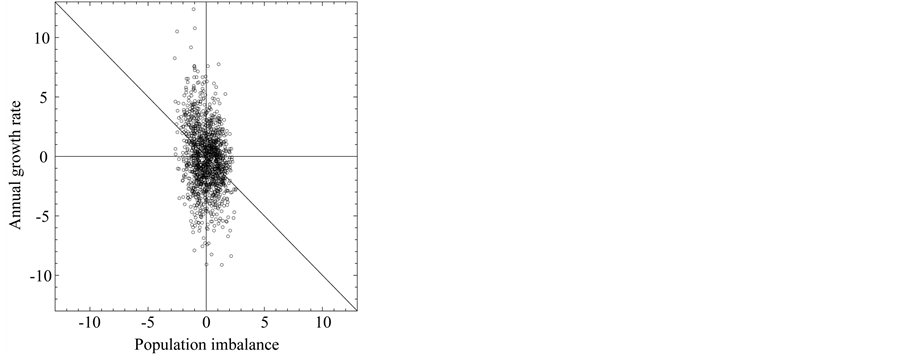
  away from the equilibrium point, the negative relationship becomes visible over the noise on time scales longer than the marginal, equilibration time. Figure 2 demonstrates that though, when plotting annual growth rate against population size, the relationship well looks like a shotgun pattern, when
 is plotted against
 , the negative feedback effects are visible, i.e.
  for
for .
.

Figure 1. Estimates of decay-time constants of the North Atlantic systems. The equilibration time Teq of each population is compared with the decay-time constants  inherent in the system and for the time-series of recruitment and catches-toescapement ratio. The solid circles refer to λ0, and the open squares (triangles) to recruitment (annual catch) variability. The dashed line represents y = x.
 (a)
(a) (b)
(b)
Figure 2. Population growth diagram of the North Atlantic fishes on fineand coarse-grained timescales. (a) The diagrams of annual growth rate (divided by total density dependence D) versus population abundance of the examined fishes are aggregated and plotted. (b) The coarse-grained diagrams demonstrate that the negative relationship is visible between Teq-year growth rate and population imbalance from equilibrium. The axes are scaled by σn. The lines represent y = −x.
After averaged over sizes  in the time-series data over
  years, the negative relationship can be seen with a predicted probability
 , whereas the dependence of
  on
on  in the data comprising
 years is rather vague (upper panels of Figure 3). Besides, I perform simulations to validate the criterion for visibility of density-dependent relationship. For simulations based on the population equation of motion (2) with the AR(1) model for the variations in the recruitment and the fishing mortality, I use parameter values that are obtained by analyzing the ICES time-series data sets. When plotting the simulated diagrams of mean growth rate versus mean abundance, conditioned on
 , for the populations observed over
  years, the data are divided into two piles; for
 , the gap between the piles is closed up (lower panels of Figure 3). Of 1000 simulations for each population, the proportion of simulations in which the negative feedback on the sample mean growth rate is observed (i.e.
 ) is plotted in Figure 4.
3. Intertwining of Stochastic Processes
In this section, I discuss the effects of multiple noise sources and noise color on measuring density dependence.
3.1. Delayed Density Dependence
Recently, Ives et al. [10] developed a pragmatic approach based on the autoregressive moving average (ARMA) model to assessment of ecological time-series, and identified the lagged structure in the data as the ARMA order. The time-lagged density-dependent effect in population fluctuations appears: the direction of annual change in population size depends on the past population trajectory.
Consider the system perturbed by multiple noise sources, where external perturbations ![]() follow AR(1) with autoregression coefficient
follow AR(1) with autoregression coefficient![]() , driven by mean-zero iid random shocks
, driven by mean-zero iid random shocks![]() , under the assumption of mutual independence of
, under the assumption of mutual independence of![]() ’s (
’s ( ; note that the results obtained in the above section can be generalized to an arbitrary number of environmental variables). Start by picking a variable
 ![]() to eliminate, and substitute
to eliminate, and substitute  into both sides of the AR(1) equation
 ; this procedure, repeated to eliminate
  one by one from the simultaneous equations, yields the ARMA
  model
model

with  -dimensional vectors
  and
and . The ARMA coefficients
 (a)
(a)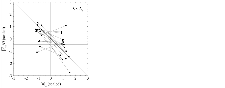 (b)
(b)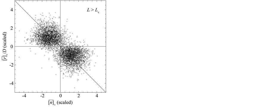 (c)
(c)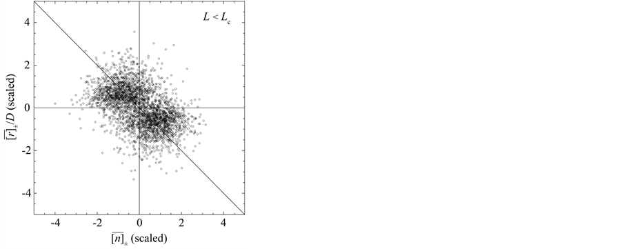 (d)
(d)
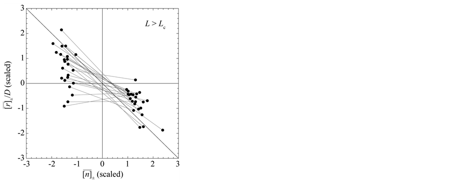
Figure 3. Mean behavior of fish populations in the North Atlantic. Shown are the diagrams (scaled by ) of mean growth rate (divided by D) versus mean abundance, conditioned on a current population imbalance
 . For the populations observed over L > Lc years (panel (a)), the negative feedback becomes statistically visible with a probability of
 . For 15 of the 38 populations examined, the time-series data comprise L < Lc years (panel (b)). In panels (c) and (d) (showing the counterparts of panel (a) and (b), respectively), the simulated growth diagrams of North Atlantic fish populations are depicted. 100 pairs for each population are piled up.
 and
and  are extracted by expanding the right-hand-side of the following pthand
  nd-degree polynomials
 (13)
(13)

Since the characteristic equation for the pth-order AR component is , the roots are found from Equation (13) to be
 ![]()
 . We see that the delayed density dependence in population dynamics arises from serial correlation in the external stochastic forcing [12] [24] .
Equation (2), transformed into the ARMA(3,1) form, gives
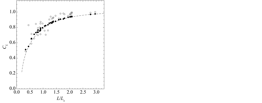
Figure 4. Degree of certainty. The values of CL are plotted against L/Lc (solid circles for the North Atlantic fish populations). The dashed line is calculated from Equation (12) with the approximation Lc = 2πTeq. The open circles read CL estimated from 1000 simulated data sets.

where ![]() denotes the differencing operation, and
denotes the differencing operation, and  is a sequence of two-dimensional independent random vectors. This third-order stochastic difference equation of population motion does not have an oscillatory solution (except for the period of two years), because
![]() ’s are restricted between ±1. Figure 1 shows that the time constant of the dominant mode (with the slowest decay rate determined by the maximum eigenvalue) disagrees with the equilibration time
’s are restricted between ±1. Figure 1 shows that the time constant of the dominant mode (with the slowest decay rate determined by the maximum eigenvalue) disagrees with the equilibration time . The differential coefficient of
  with respect to the variance
 , for fixed constant
![]() , is readily seen from Equation (5), as
, is readily seen from Equation (5), as

with

where the variance  varies linearly with the variance of
![]() . Accordingly, the equilibration time
. Accordingly, the equilibration time  is not determined solely by the eigenvalues
 ’s, but depends on the amplitude
  of population fluctuations through the driving noise
 ![]() of the AR(1) process
of the AR(1) process .
.
3.2. Noise Color
I have shown that apparently density-independent influences, which arise from colored environmental variations, modulate the population elasticity. In the following let us further analyze the impact of color of environmental variation on the total density dependence in a population. Here, for mathematical simplicity, the effects of recruitment fluctuations ![]() are only taken into account on the variance in population abundance, where the inherent elasticity
are only taken into account on the variance in population abundance, where the inherent elasticity  of the system is a given constant; the variance
  varies with the value of AR(1) coefficient
 ![]() (the variance of
(the variance of ![]() is fixed at a constant).
is fixed at a constant).
Equations (4), (5) and (7) describe the interaction between endogenous dynamics of the population and external disturbances. I demonstrate, in Figure 5, how color of recruitment variation affect the population fluctuations.
 (a)
(a)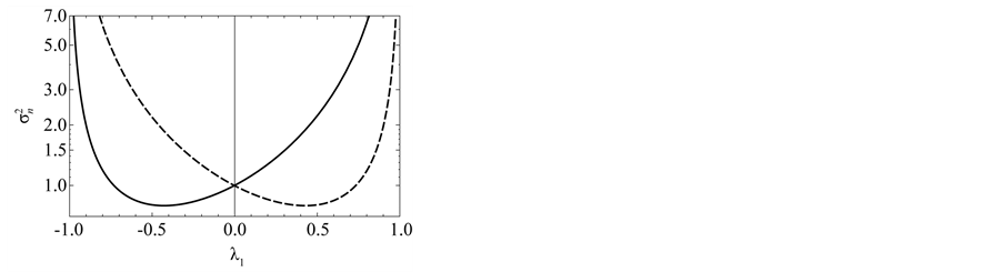 (b)
(b) (c)
(c)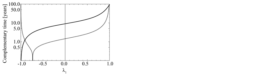 (d)
(d)
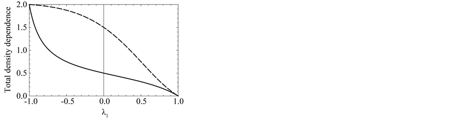
Figure 5. Effects of noise color on population processes. The total density dependence D (panel (a)), the variance  of population fluctuations (panel (b), semi-log scale), the uncertainty
  of population equilibrium (panel (c)), and the complementary time
  including the remainder term (panel (d), semi-log scale) are plotted as a function of environmental autocorrelation λ1, where L = 30 and the inherent elasticity γ of the system is fixed as
  (solid line) or −0.5 (dashed line). In panel (b),
  is divided by the variance of population process driven by white noise. In panel (d), the dotted line represents the equilibration time Teq (indicating
  for D > 1), where λ0 = 0.5.
The total density dependence D decreases when redness of noise color is increased (an increase in the autocorrelation is denoted “increased redness”), and  as
as  for any
 . The reduction in negative feedback on population growth leads to a slowing down of the equilibration process: population fluctuations have very long relaxation times and the system returns to equilibrium very slowly. In the limit
 , the population imbalance follows a random walk irrespective of the values of
 . In a blue environment,
  as
as  for any
 . In the limit
 , the system is expected to behave as
(with a mean-zero iid random variable ), which is iterated to yield
 ;
;
consequently, the amplitude jitter in the population oscillation exhibits a random-walk property and is non-stationary (regardless of the value ). In the limit
 , while the system exhibits negative feedback, the population is not regulated. Both
  lead to reduction in population regulation, resulting in unstable dynamics: the amplitude
  of population fluctuations diverges asymptotically. Either way,
  , the variance
  reaches a minimum at
 . Note from Equation (13) that when
 , the temporal correlation of population fluctuations significantly decreases (fluctuations become white in time) and the population follows rapidly mean-reverting stochastic process. The effect of an increase in redness of noise is to enhance the uncertainty in locating the population equilibrium and the complementary time. In the limit
 , we are far from the allowed certainty in measuring density dependence,
  for any
 , regardless of L. It is also confirmed that
  in both the limits
 ; while in the limit
 , the uncertainty of population equilibrium diverges less rapidly than the standard deviation of population fluctuationsi.e.
 .
.
4. Concluding Remark
Analyzing a stochastic process with slowly damped dynamics, I have derived the expression of complementarity between uncertainty in locating the population equilibrium and length of monitoring. The complementarity relation imposes a limit on the degree of certainty to which a measurement of density dependence is known. The complementarity is an essential criterion for disentangling density-dependent signals from external noise in the population process. Looking at a long time-scale makes the negative feedback on population fluctuations visible. It is difficult to know whether the system is heading toward the equilibrium point in the time-series of length less than the complementary time. This implies that density dependence is a concept that emerges from applying a proper coarse-graining procedure for time-series analysis.
The approach taken in this article is based on linear approximation of a nonlinear stochastic model. A linear approximation applies for “small” perturbations from an equilibrium point, where the “smallness” should be measured relative to the range of the uncertainty of population equilibrium. Because a large uncertainty exists in determining the population equilibrium from short observation series in ecology, it is probable that the system spends most of its time “near” the equilibrium point; a linear approximation would be usually enough accurate.
References
- Sibly, R.M. and Hone, J. (2002) Population Growth Rate and its Determinants: An Overview. Philosophical Transactions of the Royal Society of London B, 357, 1153-1170. http://dx.doi.org/10.1098/rstb.2002.1117
- Hassell, M.P., Latto, J. and May, R.M. (1989) Seeing the Wood for the Trees: Detecting Density Dependence from Existing Life-Table Studies. Journal of Animal Ecology, 58, 883-892. http://dx.doi.org/10.2307/5130
- Brook, B.W. and Bradshaw, C.J.A. (2006) Strength of Evidence for Density Dependence in Abundance Time Series of 1198 Species. Ecology, 87, 1445-1451. http://dx.doi.org/10.1890/0012-9658(2006)87[1445:SOEFDD]2.0.CO;2
- Connell, J.H. and Sousa, W.P. (1983) On the Evidence Needed to Judge Ecological Stability or Persistence. American Naturalist, 121, 789-824. http://dx.doi.org/10.1086/284105
- Hixon, M.A., Pacala, S.W. and Sandin, S.A. (2002) Population Regulation: Historical Context and Contemporary Challenges of Open vs. Closed Systems. Ecology, 83, 1490-1508. http://dx.doi.org/10.1890/0012-9658(2002)083[1490:PRHCAC]2.0.CO;2
- Solow, A.R. (1990) Testing for Density Dependence: A Cautionary Note. Oecologia, 83, 47-49. http://dx.doi.org/10.1007/BF00324632
- Beddington, J.R. and May, R.M. (1977) Harvesting Natural Populations in a Randomly Fluctuating Environment. Science, 197, 463-465. http://dx.doi.org/10.1126/science.197.4302.463
- Shepherd, J.G. and Horwood, J.W. (1979) The Sensitivity of Exploited Populations to Environmental “Noise”, and the Implications for Management. Journal du Conseil International pour l’Exploration de la Mer, 38, 318-323. http://dx.doi.org/10.1093/icesjms/38.3.318
- Ives, A.R., Dennis, B., Cottingham, K.L. and Carpenter, S.R. (2003) Estimating Community Stability and Ecological Interactions from Time-Series Data. Ecological Monographs, 73, 301-330. http://dx.doi.org/10.1890/0012-9615(2003)073[0301:ECSAEI]2.0.CO;2
- Ives, A.R., Abbott, K.C. and Ziebarth, N.L. (2010) Analysis of Ecological Time Series with ARMA(p, q) Models. Ecology, 91, 858-871. http://dx.doi.org/10.1890/09-0442.1
- Roughgarden, J. (1975) A Simple Model for Population Dynamics in Stochastic Environments. American Naturalist, 109, 713-736. http://dx.doi.org/10.1086/283039
- Royama, T. (1981) Fundamental Concepts and Methodology for the Analysis of Animal Population Dynamics, with Particular Reference to Univoltine Species. Ecological Monographs, 51, 473-493. http://dx.doi.org/10.2307/2937325
- McArdle, B.H. (1989) Bird Population Densities. Nature, 338, 628. http://dx.doi.org/10.1038/338628a0
- Lundberg, P., Ranta, E., Ripa, J. and Kaitala, V. (2000) Population Variability in Space and Time. Trends in Ecology & Evolution, 15, 460-464. http://dx.doi.org/10.1016/S0169-5347(00)01981-9
- Jonzén, N., Ripa, J. and Lundberg, P. (2002) A Theory of Stochastic Harvesting in Stochastic Environments. American Naturalist, 159, 427-437. http://dx.doi.org/10.1086/339456
- Lande, R., Engen, S., Sæther, B.-E., Filli, F., Matthysen, E. and Weimerskirch, H. (2002) Estimating Density Dependence from Population Time Series Using Demographic Theory and Life-History Data. American Naturalist, 159, 321- 337. http://dx.doi.org/10.1086/338988
- Edelstein-Keshet, L. (2005) Mathematical Models in Biology. Society for Industrial and Applied Mathematics. http://dx.doi.org/10.1137/1.9780898719147
- Shepherd, J.G. and Cushing, D.H. (1990) Regulation in Fish Populations: Myth or Mirage? Philosophical Transactions of the Royal Society of London B, 330, 151-164. http://dx.doi.org/10.1098/rstb.1990.0189
- Walters, C. and Parma, A.M. (1996) Fixed Exploitation Rate Strategies for Coping with Effects of Climate Change. Canadian Journal of Fisheries and Aquatic Sciences, 53, 148-158. http://dx.doi.org/10.1139/f95-151
- Dixon, P.A., Milicich, M.J. and Sugihara, G. (1999) Episodic Fluctuations in Larval Supply. Science, 283, 1528-1530. http://dx.doi.org/10.1126/science.283.5407.1528
- Niwa, H.S. (2006) Recruitment Variability in Exploited Aquatic Populations. Aquatic Living Resources, 19, 195-206. http://dx.doi.org/10.1051/alr:2006020
- von Neumann, J. (1941) Distribution of the Ratio of the Mean Square Successive Difference to the Variance. Annals of Mathematical Statistics, 12, 367-395. http://dx.doi.org/10.1214/aoms/1177731677
- Bulmer, M.G. (1975) The Statistical Analysis of Density Dependence. Biometrics, 31, 901-911. http://dx.doi.org/10.2307/2529815
- Kubo, R., Toda, M. and Hashitsume, N. (1991) Statistical Physics II. Nonequilibrium Statistical Mechanics. 2nd Edition, Springer-Verlag, Berlin. http://dx.doi.org/10.1007/978-3-642-58244-8
- Niwa, H.S. (2007) Random-Walk Dynamics of Exploited Fish Populations. ICES Journal of Marine Science, 64, 496- 502. http://dx.doi.org/10.1093/icesjms/fsm004
- Sparholt, H., Bertelsen, M. and Lassen, H. (2007) A Meta-Analysis of the Status of ICES Fish Stocks during the Past Half Century. ICES Journal of Marine Science, 64, 707-713. http://dx.doi.org/10.1093/icesjms/fsm038
- ICES (2008) Report of the ICES Advisory Committee, ICES Advice 2008, Books 1-10. http://www.ices.dk/publications/our-publications/Pages/ICES-Advice.aspx