Applied Mathematics
Vol.4 No.5A(2013), Article ID:31481,10 pages DOI:10.4236/am.2013.45A002
High-Order FEM Formulation for 3-D Slope Instability
1Geo-Disaster Laboratory, Graduate School of Science and Engineering, Ehime University, Matsuyama, Japan
2Graduate School of Science and Engineering, Ehime University, Matsuyama, Japan
Email: rctiwari1975@gmail.com
Copyright © 2013 Tiwari Ram Chandra et al. This is an open access article distributed under the Creative Commons Attribution License, which permits unrestricted use, distribution, and reproduction in any medium, provided the original work is properly cited.
Received February 27, 2013; revised March 13, 2013; accepted March 20, 2013
Keywords: Finite Element Method; Spectral Element Method; Slope Instability; Vegetated and Barren Slopes; Parallel Algorithm
ABSTRACT
High-order finite element method (FEM) formulation also referred to as spectral element method (SEM) formulation is currently implemented in this paper for 3-dimensional (3-D) elasto-plastic problems in stability assessment of largescale slopes (vegetated and barren slopes) in different instability conditions such as seismic and saturation. We have reviewed the SEM formulation, and have sought its applicability for vegetated slopes. Utilizing p (high-order polynomial degree or spectral degrees) and h (mesh operation for quality meshing in required elemental budgets) refining techniques in the existing FEM, the complexity of problem domain can be well addressed in greater numerical stability. Unlike the existing FEM formulation, this high-order FEM employs the same integration and interpolation points to achieve a progressive response of the instability, which drastically reduces the computational costs (formation of diagonalized mass matrix) and offers significant benefits to slope instability computations for serial and parallel implementations. With this formulation, we have achieved the following three qualities in slope instability modeling: 1) geometric flexibility of the finite elements, 2) high computational efficiency, and 3) reliable spectral accuracy. A sample problem has also been presented in this paper, which has accommodated all aforesaid numerical qualities.
1. Introduction
The high-order finite element method (FEM) is also referred to as spectral element method (SEM), which is originally applied in fluid mechanics, but is now being applied by many researchers in many fields. Because of its capacity to deliver low numerical dispersion with respect to existing finite element methods, many researchers have adopted SEM methods in seismic wave propagation analysis (e.g., [1-10]). The SEM method combines the flexibility of FEM with the accuracy of a spectral approach, adopting the hexahedral elements satisfactorily, which represents the complexities of problem domain. The domain of the hexahedral elements is discretized using high-degree Lagrange interpolants, and integration over an element is accomplished based on the GaussLobatto-Legendre (GLL) integration rule. A combination of discretization and integration effort results in a diagonalized mass matrix, which drastically reduces the computation effort, and supports parallel implementation, which demonstrates the most effective and efficient method among all methods currently in use for slope instability computations. In this context, a use of SEM in slope instability has been made for the first time by Gharti et al. [11], in elasto-plastic framework (i.e., Specfem 3d Geotech, an open source package). This paper further implements the SEM package for vegetated slope stability incorporating root reinforcement formulation. With this formulation, the role of vegetation in soil slope stability can be justified analytically and numerically.
The advantage of SEM over existing FEM is in the use of high-order basis functions. High-order elements are well established in geotechnical FEM (e.g., 15 node triangles), but the computational burden is not addressed by any existing FEM methods. The advantage of forming a diagionalized mass matrix for a pseudo-static analysis is, in fact, not sufficient. However, this paper finds a broader scope for pseudo-static applications for vegetated and barren slope instability, and predicts reliable values of safety factors through certain refinement techniques, i.e., p-increase in spectral degree and h-increase in elemental budgets, and ensuring the quality mesh in the SEM. It investigates the application of SEM to 3-D slope instability analysis in elasto-plastic framework. As an application, this paper utilizes the same source package to demonstrate the stability aspects of vegetated and barren slope in different instability conditions such as seismic and saturation.
2. Mathematical Foundation
2.1. High-Order FEM Formulation
Traction or stress vector  can be written in tensor notation as per Cauchy’s formula as follows.
 (1)
(1)
where,  and
and  are known respectively as the Cauchy stress tensor and unit outward normal to the boundary.
According to Newton’s Law of conservation of linear momentum, the time rate of change of linear momentum of particles equals the net force exerted on them, which is expressed as follows.
 (2)
(2)
where,  and
and  are respectively the mass of the particle, its velocity, and net force acting on the particle. For an arbitral (sub) domain
  of a solid continuum of density
  subjected to body forces (per unit volume)
  and surface forces (per unit area)
  acting on the boundary
  the principle of conservation of linear momentum can be written as follows.
 (3)
(3)
where,  is known as the displacement vector. Using the Cauchy’s formula, the Equation (3) can be written as both tensor form and general elaborated form.
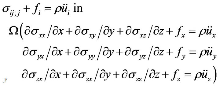 (4)
(4)
where,  is known as the particle acceleration. We use a semicolon (;) for covariant differentiation. The generalized Hooke’s Law can be written in the following form.
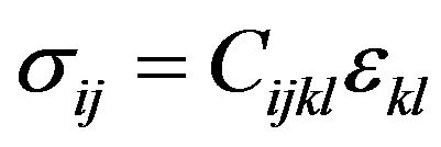 (5)
(5)
where,  is known as elasticity tensor for linearly elastic isotropic material, i.e.,
and  is known as mass density, i.e.,

here,  and
and  are known respectively as the weight and density function of soil material [12]. These two expressions include root reinforcement effect of vegetation, where
  and
and  are known respectively as weight function of roots, weight function of soil, density of roots, density of soils, and root area ratio (RAR). RAR denotes the fraction of soil cross-section occupied by roots
 An additional cohesion due to the presence of roots can be calculated by two major characteristics of root systems
  (average tensile strength of root fibers), and RAR. Both
  and RAR are influenced by species and site factors such as local climate, soil type, season, root type and size as well as root architecture (e.g., [13,14]). Using perpendicular root reinforcement model, the additional root cohesion
  can be computed by the following relation as follows.
 (6)
(6)
where,  and
and  are known respectively as the common coefficient factor and a mobilized tensile strength of root fibers as follows.
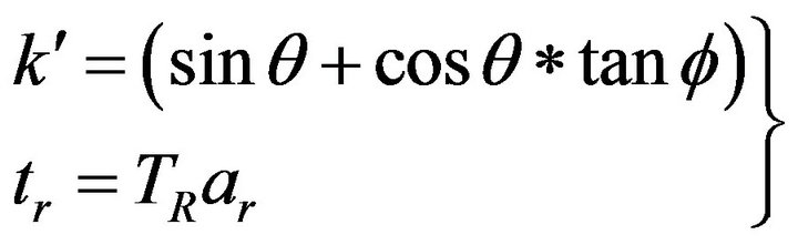 (7)
(7)
where,  and
and  are known respectively as the angle of shear distortion in shear zone and angle of internal friction of soil. The common value of
  can be taken as 1.15 [15] or 1.2 [16]. To account the variability of root diameter, expression
  can be further written as follows.
 (8)
(8)
where,  and
and  are known respectively as the tensile strength of root and RAR, both specified per diameter class
  and
and  is the number of class considered [17].
Soil is considered as anisotropic material (soil material properties varies in all direction). The symmetry of Cauchy’s stress tensor  and the generalized expression of Hooke’s Law (Equation (5)) implies that
  In the above expression (5),
  and
and  are respectively known as fourth-order elasticity tensor and Cauchy strain tensor.
In tensor form, the Cauchy strain can be further written as follows.
 (9)
(9)
Further, the Equation (4) first expresses to weighted integral form and then follows integration by parts and rearranges the expressions simultaneously in the following form [18].
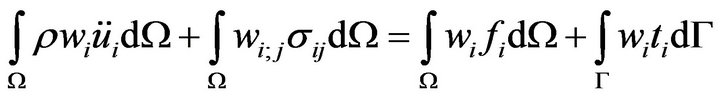 (10)
(10)
The Equation (10) is the weak form of the governing equation, where,  and
and  are known respectively as the volume of the domain and boundary of the domain. The next step would be the use of Lagrange interpolation function and find out the displacement field as per spectral element approach. Interpolation functions in both local (e.g.,
  denotes for origin and
 denotes for certain positive
 “
“ ” distance), and natural (e.g., denotes for origin and
  for positive “
 ” coordinate, “
 ” and
” and  for negative “
 ” coordinate, “
 ”) coordinates are as follows.
 (11)
(11)
We have used Gauss-Legendre-Lobatto (GLL) interpolation points  of polynomial of degree
  by the relation,
  in each direction of element. The expansion of any element is accomplished based on Lagrange polynomials of suitable degree
  constructed for
  interpolation nodes. The total number of interpolation points is the product of the number of GLL points along each direction,
 . The work interpolation is carried out using Lagrange polynomials defined on the GLL points to obtain the progressive response of displacement field. It needs to evaluate the displacement, its spatial derivatives, and integrals encountered in the weak formulation in those nodes. With this technique, each element of the mesh contains
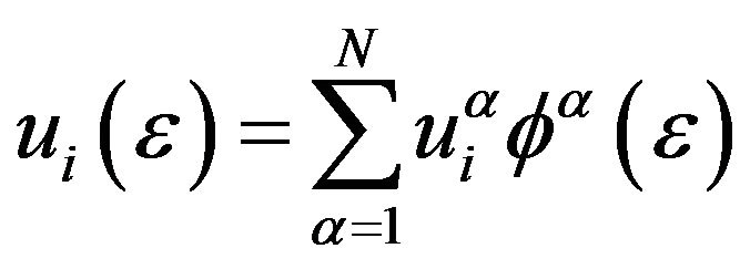
  GLL points, where grid points that lie on the sides, edges, or corners of an element are shared amongst neighboring elements of the domain (e.g.,
  , total GLL points = 64 Nos.). The displacement field (i.e., computations of displacement) as per the SEM can be expressed as follows (i.e., similar displacement function as uses in FEM formulation, i.e.,
 ).
).
 (12)
(12)
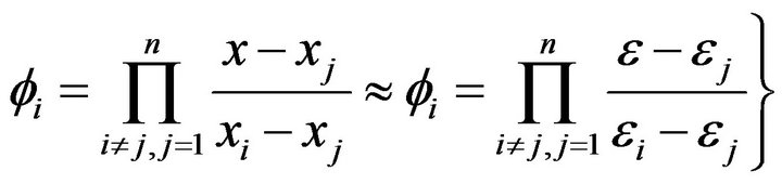
where, the interpolation function  in natural coordinates is, determined by the tensor product of 1-D Lagrange polynomials as follows.
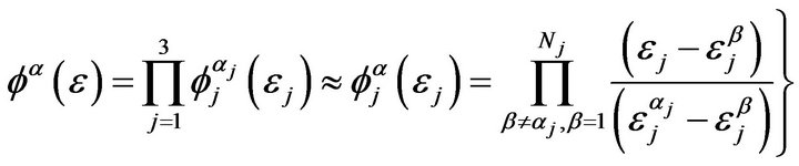 (13)
(13)
where,  is the index of a GLL point located at
  For this numerical integration, a point
  in a deformed element is mapped to a point
 in the natural element as follows.
 (14)
(14)
where,  and
and  are known respectively as a shape function, and
  is the number of geometrical nodes
  of an element. The GLL points are used as quadrature points (integration points) for this numerical integration. A quadrature rule is an approximation of the definite integral of a function, usually stated as a weighted sum of function values at specified points within the domain of integration. The most important issue of SEM is the use of GLL quadrature for spatial integration, using the same points for interpolation and integration, and formation of diagonalized mass matrix. The SEM is a continuous Galerkin method, in which the interpolation function
  is taken as the test function
  Substituting the value of
  in the Equation (12), we obtain the following relation [18].
 (15)
(15)
Substituting the value of  in the weak formulation, this equation turns as follows [17].
 (16)
(16)
In the Equation (16),  and
and  are known respectively as the acceleration and displacement vectors. Similarly,
  and
and  are known respectively as the mass matrix, stiffness matrix and force vector of an element, and are given as follows.
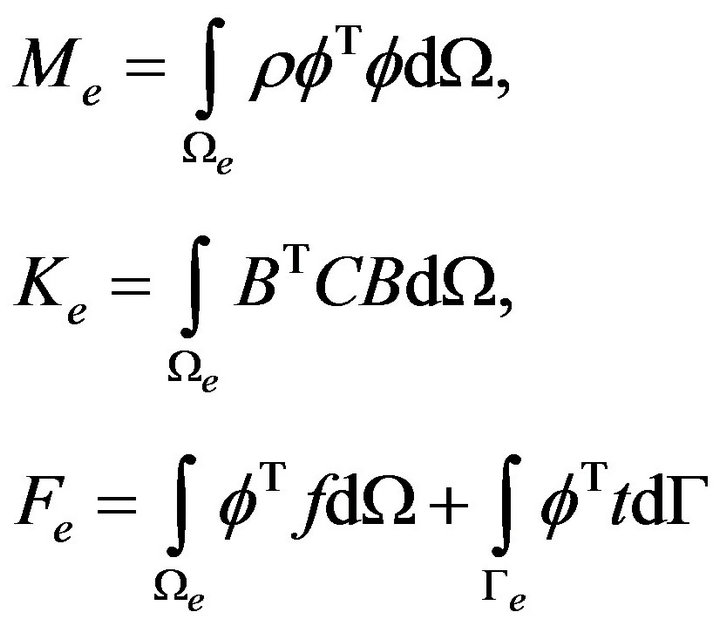
where,  and
and  are known respectively as transpose and volume of an element. Other notations such as,
  and
and  are known respectively as the interpolation function matrix, the strain-displacement matrix, and elasticity matrix. With these considerations, the elemental mass matrix can be further written as follows [18].
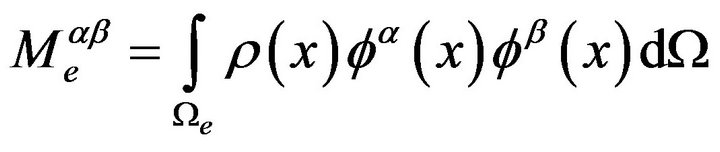 (17)
(17)
In this relation,  and
and  vary from 1 to
  The elemental mass matrix can be further expressed with the integration based on GLL quadrature over the GLL points as follows [18].
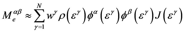 (18)
(18)
where,  and
and  are known respectively as the integration weights and the determinants of the Jacobian matrix evaluated at the
  integration point. The elemental mass matrix can be further expressed with using the orthogonality of the interpolation function in the following relation [18].
 (19)
(19)
In the above expression,  represents the Kronecker delta
  that simplifies the mathematical problem. Therefore, the elemental mass matrix is diagonal, which is true for global mass matrix. This facilitates an effective time-marching scheme, which is a significant advantage of the SEM over the existing FEM. A set of global equation can be obtained by assembling the elemental equations [18].
 (20)
(20)
where,  and
and  are known respectively as global displacement vector, global stiffness vector and global force vector (
 : elemental stiffness matrix,
 : elemental force matrix). This formulation can only address the time-dependent elasto-plastic problems relevant to slope instability in the following form.
 (21)
(21)
The scope of SEM is in dynamic slope instability problems; however, it offers significant benefits to static slope instability from computational point of view. The SEM is an elegant formulation of the FEM with a high degree piecewise polynomial basis (high-order FEM). The major difference between the existing FEM and SEM is in the choice of the basis (form) functions inside the elements in which the fields are described. Displacement function is expressed in each element in terms of high-degree Lagrange interpolants (polynomials). The integrals are then composed based on GLL quadrature points, which are used to form an exact diagonal matrix, and are therefore simplified the algorithm. In this formulation, both integration point and interpolation point lie in the same point that ensures the reduction of interpolation effort for the displacement and stress computation (Figure 1), and leads to fast and exact solution with greater numerical stability.
To address the different degree of soil saturation and pore-water pressure, the following relation can be applied in aforesaid formulation [18].
 (22)
(22)
where,  denotes the water pressure computed from simple hydrostatic relation (
 : unit weight of water,
 : depth of water column).
2.2. Strength Reduction Technique
The shear strength reduction technique is first proposed by Zienkiewicz et al. [19], and is further extended to achieve the safety factor for the slope instability assessment by different researchers (e.g., [20-25]). In this technique, an application of gravity loading is followed by a systematic reduction in soil strength until failure occurs, which is achieved using a strength reduction factor (SRF), to the frictional and cohesive components of strength in the form of factored frictional  and cohesive component
  in the basic equation of
 (23)
(23)
At certain stage of computation, Gauss points undergo plastic deformation, which requires a large number of
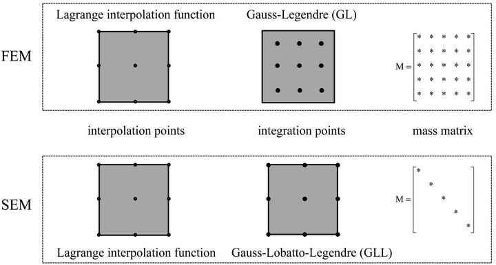
Figure 1. Diagrammatical interpretation of solution procedure for FEM and SEM.
iterations for the convergence of the results. We consider it as failure stage, and consider factor of safety (FOS) to that stage of SRF.
3. Spectral Element Discretization
SEM works primarily on hexahedral elements. Each hexelement contains at least 20 nodes in 6 faces for nonlinear problems, however, we have worked on symmetric node numbers (GLL points, i.e.,  , where
  represents the polynomial degree) of 2, 3, 4, 5 etc., in each direction (i.e., X, Y, and Z) of the problem domain that respectively equivalent to 8, 27, 64, 125 by a simple relationship
  The governing equations of non-linear problems contain high-degree of polynomials or power terms to capture the complexities of the problem domain. The non-linear solution thus required also demands huge number of iteration. SEM discretization, as shown in Figure 2, has great influence on numerical stability. Poor quality mesh creates numerical instability (i.e., increase in the computational cost, lack of convergence, and the inaccuracy of the results). Different researchers have worked on hexahedral meshing and have emphasized on quality meshing for greater numerical stability (e.g., [26-29]). The successful application of the SEM includes the effective mesh operation, which includes descretization and mapping. SEM discretization follows five steps: 1) the domain is split into hexahedral, 2) each sub-domain is mapped into a reference element, 3) NGL nodes are then introduced, 4) spectral grid points are then mapped back into the domain, and 5) whole domain is mapped with spectral grid points (Figure 2).
4. An Application to Large-Scale Slope Instability Modeling
As an application to large-scale slope instability, we have used a newly released open-source program SPECFEM3D_GEOTECH along with mesh generating toolkit, CUBIT [30] and result visualization tool, Paraview [31]. With this implementation, we have ensured the reliable results in less and less computational burden using hand p-refinement techniques. We have found a reliable result at 3 GLL points and 10,000 hexahedron elements with quality meshing operation followed as per the SEM technique. The results show that this package works efficiently to large and complex slope instability problems of different degree of complexities. The program efficiently uses fully unstructured hexahedral meshes, and shows capacity of discretizing the problem domain. We have successfully used the program in parallel implementation (using Message passing interface, MPI [32] and partitioning tool, SCOTCH [33]) for Linux platform of 4- processor computer, and have dealt with partially and fully saturated soil slope condition along with pseudostatic seismic condition for vegetated and barren soil slopes. In this formulation, we have employed initial and final water table to the model so that the program counted partially saturated slopes, and water pressure acted in the wet region of the slope along with gravity
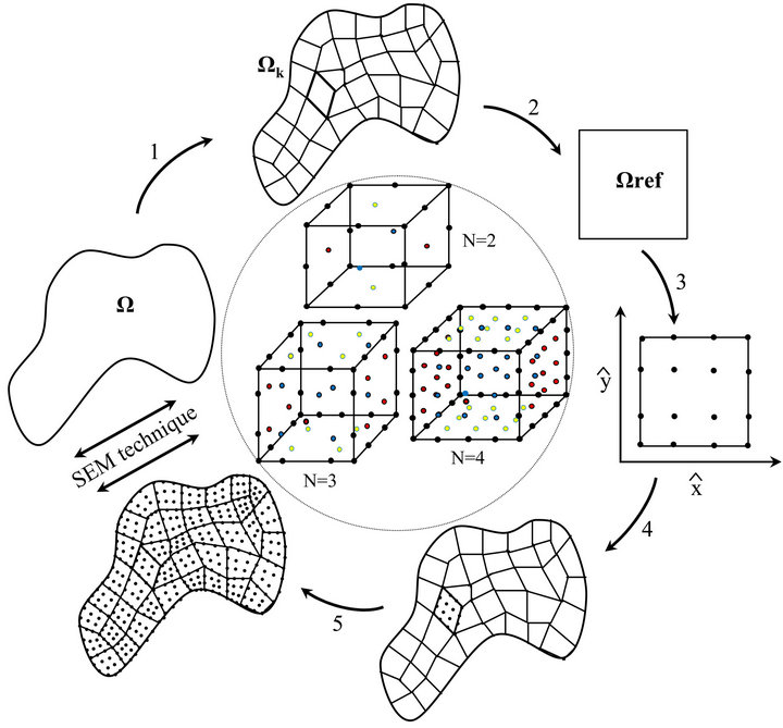
Figure 2. Spectral element discretization technique.
load that reduced the soil strength parameters. It considers a homogenous soil layer below and above the water table, which considered the same material properties with or without considering the soil saturation effects. The meshing effort accommodates the submerged meshes while calculating the hydrostatic pressure. It easily identifies submerged nodes of uniform meshing sizes; however, it considers inaccurately when the water table touched the mesh of sharp corners. With this accommodation, we have observed a complete ground water fluctuation effect on soil slope instability, which we have used to evaluate the stability of slopes in possible slope stability enhancement projects.
Figure 3(a) shows a typical model for large-scale slope instability of slope layer height,  (m), slope length,
  (m), slope breadth,
  (m), and slope angle
  (degrees). We have considered root depth of
  (m), and have assumed the water table positions to be at every single meter height of the slope layer (i.e.,
  to 5 m). We have considered horizontal seismic coefficient,
  of 0.10 g for a severe earthquake event as per Terzaghi [34]. Figure 3(b) and Figure 3(c) represent respectively the hexahedron meshing model in 3D, and domain decomposition into 4 subdomains. Figure 3(d) represents the typical displacement field of 4 representative safety factors of 1.05, 1.10, 1.15, and 1.20 in case of slope material model of ML along with root-cohesion of 20 kN/m2, and water table position of
  m. The results show that there is distinct change in displacement at SRF of 1.15 and 1.20, which indicates the possible safety factor for that computation. Computations proceeds in each case of slope instability prepared for different soil slope material conditions as in Table 1. This computational framework adopts modulus of elasticity
 and poissons ratio
  respectively of 11000 kN/m2 and 0.3 for silty sand, many fines (SM-ML)
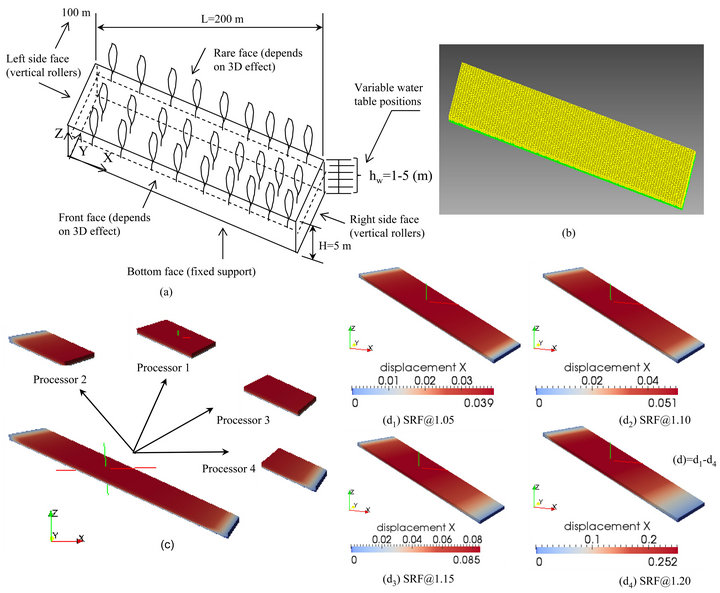
Figure 3. Typical slope instability modeling: (a) schematic diagram of slope model; (b) hexahedral meshing in CUBIT; (c) domain decomposition to 4 sub-domains, and (d) displacement field of soil material model ML (as per USCS category) at SRF 1.05, 1.10, 1.15, and 1.20.

Table 1. Average geotechnical soil parameter of 8 soil types (as per USCS category) adopted by Krahenbuhl and Wagner [35].
to silt (ML), and respectively of 8500 kN/m2 and 0.325 for silt to clayey soil (CL-ML) to clay (CH), as per the common practice of soil parameters followed in geotechnical FEM. Figure 4(a) shows the comparative instability conditions with 8 soils as per USCS category at water table position 1 m from the bottom of soil layer (i.e,  m). Results show respectively that 3 soil types, such as CL-ML, CL, and CH perform higher safety factors of 1.4, 1.45, and 1.60; 2 soil types SM-SC and SC-CH perform average safety factors of 1.10 and 1.15; 2 soil types SC-CL and ML perform critical safety factor of 1.0, and remaining soil type SM-ML performs unstable safety factor of 0.85 with the slope model considered (Table 2). Figure 4(b) shows 4 instability cases (i.e., C1 - C4) of slope model for soil type of ML. Results confirm that slope model performs highly unstable condition in case of dry water table and dry and wet season (partial and full saturation) seismic condition as well as wet season static condition, however, slope performs fairly stable result with dry static and dry season static cases (Table 3). Computations show that fully saturated seismic soil slope condition is the worst scenario of slope instability and slope model increases FOS significantly in the case of lowering the water table to a significant depth (Figure 4(c), and corresponding Table 4).
Figure 5(a) shows the effect of root-reinforcement on FOS. The computation suggests the slope performs considerable stability with increase in root cohesion in case of low level water table position (e.g.,  m). The contribution of root-reinforcement in slope stability can only be achieved with fairly stable soil slope conditions. The contribution of root cohesion can only be effective in dry season static conditions of the slope model considered (Table 5). Theoretically, it performs the positive effect on slope stability whatever the degree of instability existed within the modeled domain; however, the stability greatly depends on geometry of the slope model as compared to possible contribution by root-cohesion. Figure 5(b) indicates elastic and plastic iterations for elastoplastic modeling. It shows that elastic and plastic parts of the curve respectively, which require less and high number of iterations for the convergence of the results. We observe FOS respectively of 1.10 in first 2 root-cohesions (i.e.,
  kN/m2 and
  kN/m2) and 1.15 in case of remaining root cohesion values (i.e.,
  kN/m2 and
  kN/m2), which indicate the influence of slope geometry and soil material properties on slope stability than with root-reinforcement, however, its effect on slope stability is no longer excluded in the analysis because the contribution of root-reinforcement solely depends on as model. With this accommodation, the safety factors thus obtained in each possible case have become the best possible measurements to evaluate the stability of various stages of landslides. With the application of h (i.e., mesh, elemental budgets) and p (i.e., spectral degree, degree of interpolation, GLL points) refinement techniques, SEM performs to be an efficient method over the existing FEM.
5. Conclusion
SEM formulation allows the simulation of the complicated stress-strain behavior of soils, which can cope with irregular geometries, complex boundary conditions, and pore-water pressure regimes in large-scale problem domain of vegetated and barren slopes. With application of h- (i.e., mesh, elemental budgets), and p (i.e., spectral degree, degree of interpolation, GLL points) refinement techniques, SEM performs to be an efficient method over the existing FEM. It relates with high-order FEM that can capture the complexity of the problem domain, and forms the diagonalized mass matrix, which significantly reduces the computation burden. As an application of SEM, we have utilized a recently released open source program SPECFEM3D_GEOTECH, which has capacity of simulating progressive failure in 3D for large-scale
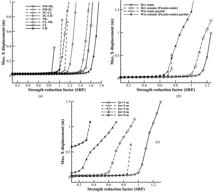
Figure 4. Displacement versus SRFs: (a) 8 soil material models from SM-ML to CH (as per USCS soil category) in case of hw = 1 m; (b) seismic (Kx = 0.1 g) and saturation (hw = 1 m) condition of soil material model ML (as per USCS category), and (c) ground water fluctuations effect on slope instability at water table positions, hw, of 1.0 m, 2.0 m, 3.0 m, 4.0 m, and 5.0 m from the bottom of soil surface of same material model of ML.

Table 2. Summary of the FOS in different soil material models as per USCS category.
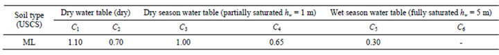
Table 3. Summary of FOS in different instability cases.
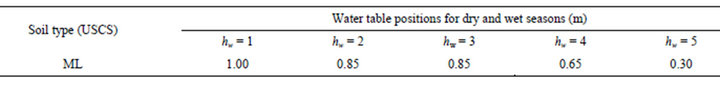
Table 4. Summary of the FOS for different water table positions in static condition.

Figure 5. Root-reinforcement effect (soil slope model of USCS soil ML at hw = 1 m): (a) displacement (m) versus SRFs, and (b) non-linear iteration (Nos.) versus SRFs.
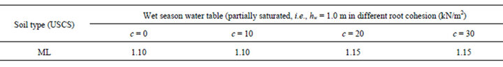
Table 5. Summary of the FOS for dry season water table (i.e., hw = 1.0 m) in different root-cohesion.
problem domain in various cases of instability. The computations have carried out from several possible strength reduction factors (SRFs) to find out the reliable FOS from trial SRFs on the basis of abrupt change in displacement. We have successfully performed the role of following parameters on slope stability: 1) material properties; 2) seismic and saturation conditions; 3) water table positions; and 4) root-reinforcements. Computations suggest that root-reinforcement effect contributes significantly on dry season slope stability (static condition). The geometry of problem domain along with soil material properties have greater role on slope stability. With this simple implementation, it has evidenced that the benefit of SEM over FEM approach can be well examined in large and complex modeling domains of vegetated and barren slopes too.
6. Acknowledgements
The authors would like to acknowledge the valuable comments and suggestions provided by Prof. Padma Bahadur Khadka, Tribhuvan University Nepal.
REFERENCES
- P. Cupillard, E. Delavaud, G. Burgos, G. Festa, J. P. Vilotte, Y. Capdeville and J. P. Montagner, “RegSEM: A Versatile Code Based on the Spectral Element Method to Compute Seismic Wave Propagation at the Regional Scale,” Geophysical Journal International, Vol. 188, No. 3, 2012, pp. 1203-1220. doi:10.1111/j.1365-246X.2011.05311.x
- D. Jonas, D. Basabe and M. K. Sen, “Stability of the High-Order Finite Elements for Acoustic or Elastic Wave Propagation with High-Order Time Stepping,” Geophysical Journal International, Vol. 181, No. 1, 2010, pp. 577-590. doi:10.1111/j.1365-246X.2010.04536.x
- I. Khan and B. H. V. Topping, “Parallel Finite Element Analysis Using Jacobi-35 Conditioned Conjugate Gradient Algorithm,” Advances in Engineering Software, Vol. 25, No. 2-3, 1996, pp. 309-319. doi:10.1016/0965-9978(95)00111-5
- J. Y. Kim and S. R. Lee, “An Improved Search Strategy for the Critical Slip Surface Using Finite Stress Fields,” Computers and Geotechnics, Vol. 21, No. 4, 1997, pp. 295-313. doi:10.1016/S0266-352X(97)00027-X
- D. Komatitsch and J. Tromp, “Introduction to the Spectral Element Method for Three-Dimensional Seismic Wave Propagation,” Geophysical Journal International, Vol. 139, No. 3, 1999, pp. 806-822. doi:10.1046/j.1365-246x.1999.00967.x
- D. Komatitsch and J. Tromp, “Spectral-Element Simulations of Global Seismic Wave Propagation I. Validation,” Geophysical Journal International, Vol. 149, No. 2, 2002, pp. 390-412. doi:10.1046/j.1365-246X.2002.01653.x
- D. Komatitsch, S. Tsuboi and J. Tromp, “The SpectralElement Method in Seismology. Seismic Earth: Array Analysis of Broadband Seismograms,” Geophysical Monograph Series, Vol. 157, 2005, pp. 205-227. doi:10.1029/156GM13
- D. Komatitsch and J. P. Vilotte, “The Spectral Element Method: An Efficient Tool to Simulate the Seismic Response of 2D and 3D Geological Structures,” Bulletin of the Seismological Society of America, Vol. 88, No. 2, 1998, pp. 368-392.
- R. Pasquetti and F. Rapetti, “Spectral Element Methods on Unstructured Meshes: Comparisions and Recent Advances,” Journal of Scientific Computing, Vol. 27, No. 1-3, 2006, pp. 377-387. doi:10.1007/s10915-005-9048-6
- J. Tromp, D. Komatitsch and Q. Liu, “Spectral-Element and Adjoint Methods in Seismology,” Communications in Computational Physics, Vol. 3, No. 1, 2008, pp. 1-32.
- H. N. Gharti, D. Komatitsch, V. Oye, R. Martin and J. Tromp, “Specfem 3D Geotech User Manual, 1.1 Beta,” 2012. http://www.geodynamic.org/cig/software/specfem3d-geotech
- R. C. Tiwari, N. P. Bhandary, R. Yatabe and D. R. Bhat, “New Numerical Scheme in the Finite Element Method for Evaluating Root-Reinforcement Effect on Soil Slope Stability,” Geotechnique, Vol. 63, No. 2, 2013, pp. 129- 139. doi:10.1680/geot.11.P.039
- M. Genet, A. Stokes, F. Salin, S. B. Mickovski, T. Fourcaud, J. Dumail and L. P. H. Van Beek, “The Influence of Cellulose Content on Tensile Strength in Tree Roots,” Plant and Soil, Vol. 278, No. 1-2, 2005, pp. 1-9.
- D. H. Gray and R. D. Sotir, “Biotechnical Soil Bioengineering Slope Stabilization: A Practical Guide for Erosion Control,” John Wiley & Sons Ltd., New York, 1996.
- L. J. Waldron, “The Shear Resistance of Root-Permeated Homogenous and Stratified Soil,” Soil Science Society of America Journal, Vol. 41, No. 5, 1977, pp. 843-849. doi:10.2136/sssaj1977.03615995004100050005x
- T. H. Wu, M. C. Kinnell, W. P. McKinnell III and D. N. Swanston, “Strength of Tree Roots and Landslides on Prince of Wales Island,” Canadian Geotechnical Journal, Vol. 16, No. 7, 1979, pp. 19-33. doi:10.1139/t79-003
- G. B. Bischetti, E. A. Chaiaradia, T. Epis and E. Morlotti, “Root Cohesion of Forest Species in the Italian Alps,” Plant and Soil, Vol. 324, No. 1, 2009, pp. 71-89. doi:10.1007/s11104-009-9941-0
- H. N. Gharti, D. Komatitsch, V. Oye, R. Martin and J. Tromp, “Application of an Elastoplastic Spectral-Element Method to 3D Slope Stability Analysis,” International Journal for Numerical Methods in Engineering, Vol. 91, No. 1, 2012, pp. 1-26. doi:10.1002/nme.3374
- O. C. Zienkiewicz, C. Humpheson and R. W. Lewis, “Associated and Non-Associated Visco-Plasticity and Plasticity in Soil Mechanics,” Geotechnique, Vol. 25, No. 4, 1975, pp. 671-689. doi:10.1680/geot.1975.25.4.671
- M. M. Berilgen, “Investigation of Stability of Slopes under Drawdown Conditions,” Computers and Geotechnics, Vol. 34, No. 2, 2007, pp. 81-91. doi:10.1016/j.compgeo.2006.10.004
- D. V. Griffiths, J. Huang and G. F. Dewolfe, “Numerical and Analytical Observations on Long and Infinite Slopes,” International Journal for Numerical and Analytical Methods in Geomechanics, Vol. 35, No. 5, 2011, pp. 569-585. doi:10.1002/nag.909
- D. V. Griffiths and P. A. Lane, “Slope Stability Analysis by Finite Elements,” Geotechnique, Vol. 49, No. 3, 1999, pp. 387-403. doi:10.1680/geot.1999.49.3.387
- M. S. Huang and C. Q. Jia, “Strength Reduction FEM in Stability Analysis of Soil Slope Subjected to Transient Unsaturated Seepage,” Computer and Geotechnics, Vol. 36, No. 1-2, 2009, pp. 93-101. doi:10.1016/j.compgeo.2008.03.006
- P. A. Lane and D. V. Griffiths, “Assessment of Stability of Slopes under Draindown Conditions,” Journal of Geotechnical and Geoenvironmental Engineering (ASCE), Vol. 126, No. 5, 2000, pp. 443-450.
- T. Matsui and K. C. San, “Finite Element Slope Stability Analysis by Strength Reduction Technique,” Soils and Foundation, Vol. 32, No. 1, 1992, pp. 59-70. doi:10.3208/sandf1972.32.59
- D. Peter, D. Komatitsch, Y. Luo, R. Martin, N. Le Goff, E. Casarotti, P. Le Loher, F. Magnoni, Q. Liu and Peeligrini, “SCOTCH User’s Guide Version 5.1,” 2010. http://www.labri.fr/perso/pelegrin/scotch/
- M. A. Price and C. G. Armstrong, “Hexahedral Mesh Generation by Medial Surface Subdivision: Part II. Solids with Flat and Concave Edges,” International Journal for Numerical Methods in Engineering, Vol. 40, No. 1, 1997, pp. 111-136. doi:10.1002/(SICI)1097-0207(19970115)40:1<111::AID-NME56>3.0.CO;2-K
- J. Shepherd and C. Johnson, “Hexahedral Mesh Generation Constraints,” Engineering with Computers, Vol. 24, No. 3, 2008, pp. 195-213. doi:10.1007/s00366-008-0091-4
- T. J. Tautges, “The Generation of Hexahedral Meshes for Assembly Geometry: Survey and Progress,” International Journal for Numerical Methods in Engineering, Vol. 50, No. 12, 2001, pp. 2617-2642. doi:10.1002/nme.139
- CUBIT Development Team, “CUBIT Mesh Generation Environment Volume 1 User’s Manual,” Sandia National Lab, 1999. http://cubit.sandia.gov/cubitprogram.html
- Paraview Develops Team, “Paraview,” Kitware Inc., Clifton Park, 2010. http://paraview.org/wiki/paraview
- Open MPI Team, “The Open MPI Project, Indiana University,” Bloogminton, 2011. http://www.open-mpi.org
- Peeligrini, “SCOTCH User’s Guide Version 5.1,” 2010. http://www.labri.fr/perso/pelegrin/scotch/
- K. Terzaghi, “Mechanisms of Landslides,” Geotechnical Society of America, Berkeley, 1950, pp. 83-125.
- J. Krahenbuhl and A. Wagner, “Survey, Design, and Construction of Trail Suspension Bridges for Remote Areas, SKAT,” Swiss Center for Appropriate Technology, St. Gallen, 1983.