ABSTRACT

Teaching-Learning-Based Optimization (TLBO) is recently being used as a new, reliable, accurate and robust optimization technique scheme for global optimization over continuous spaces [1]. This paper presents an, improved version of TLBO algorithm, called the Weighted Teaching-Learning-Based Optimization (WTLBO). This algorithm uses a parameter in TLBO algorithm to increase convergence rate. Performance comparisons of the proposed method are provided against the original TLBO and some other very popular and powerful evolutionary algorithms. The weighted TLBO (WTLBO) algorithm on several benchmark optimization problems shows a marked improvement in performance over the traditional TLBO and other algorithms as well.

1. Introduction

In evolutionary algorithms the convergence rate of the algorithm is given prime importance for solving an optimization problem. The ability of the algorithm to obtain the global optima value is one aspect and the faster convergence is the other aspect. It is studied in the evolutionary techniques literature that there are few good techniques, often achieve global optima results but at the cost of the convergence speed. Those algorithms are good candidates for use in the areas where the main focus is on the quality of results rather than the convergence speed. In real world applications, the faster computation of accurate results is the ultimate aim. In recent time, a new optimization technique called Teaching learning based optimization [1] is gaining popularity [2-8] due to its ability to achieve better results in comparatively faster convergence time to techniques like Genetic Algorithms (GA) [9,10], Particle swarm Optimizations (PSO) [11-17] Differential Evolution (DE) [18-20] and some of its variants like DE with Time Varying Scale Factor (DETVSF), DE with Random Scale Factor (DERSF) [21] etc. The main reason for TLBO being faster to all other contemporary evolutionary techniques is it has no parameters to tune. However, in evolutionary computation research there has been always attempts to improve any given findings further and further. This work is an attempt to improve the convergence characteristics of TLBO further without sacrificing the accuracies obtained in TLBO and in some occasions trying to even better the accuracies.

In our proposed work, the attempt is made to include a parameter called as “weight” in the basic TLBO equations. Our proposed algorithm is known as weighted TLBO (WTLBO). The philosophy behind inclusion of this parameter is justified in Section 3 of the paper. The inclusion of this parameter is found not only bettering the convergence speed of TLBO, even providing better results for few problems. The performance of WTLBO for solving global function optimization problems is compared with basic TLBO and other evolutionary techniques. It can be revealed from the results analysis that our proposed approach outperforms all approaches investigated in this paper.

The remaining of the paper is organized as follows: in Section 2, we give a brief description of TLBO. In Section 3, we describe the proposed Weighted TeachingLearning-Based Optimizer (WTLBO). In Section 4, experimental settings and numerical results are given. The paper concludes with Section 5.

2. Teaching-Learning-Based Optimization

This optimization method is based on the effect of the influence of a teacher on the output of learners in a class. It is a population based method and like other population based methods it uses a population of solutions to proceed to the global solution. A group of learners constitute the population in TLBO. In any optimization algorithms there are numbers of different design variables. The different design variables in TLBO are analogous to different subjects offered to learners and the learners’ result is analogous to the “fitness”, as in other population-based optimization techniques. As the teacher is considered the most learned person in the society, the best solution so far is analogous to Teacher in TLBO. The process of TLBO is divided into two parts. The first part consists of the “Teacher Phase” and the second part consists of the “Learner Phase”. The “Teacher Phase” means learning from the teacher and the “Learner Phase” means learning through the interaction between learners. In the sub-sections below, we briefly discuss the implementation of TLBO.

2.1. Initialization

Following are the notations used for describing the TLBO:

N: number of learners in a class i.e. “class size”;

D: number of courses offered to the learners;

MAXIT: maximum number of allowable iterations.

The population X is randomly initialized by a search space bounded by matrix of N rows and D columns. The parameter of the learner is assigned values randomly using the equation

(1)

where rand represents a uniformly distributed random variable within the range (0,1), and represent the minimum and maximum value for parameter. The parameters of learner for the generation g are given by

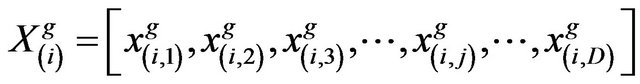(2)

2.2. Teacher Phase

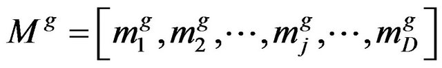
The mean parameter of each subject of the learners in the class at generation is given as

(3)

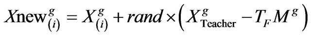
The learner with the minimum objective function value is considered as the teacher for respective iteration. The Teacher phase makes the algorithm proceed by shifting the mean of the learners towards its teacher. To obtain a new set of improved learners a random weighted differential vector is formed from the current mean and the desired mean parameters and added to the existing population of learners.

(4)

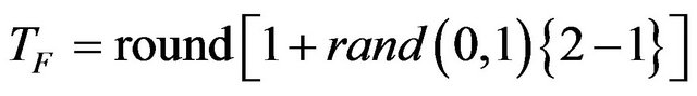
is the teaching factor which decides the value of mean to be changed. Value of can be either 1 or 2. The value of is decided randomly with equal probability as,

(5)

where is not a parameter of the TLBO algorithm. The value of is not given as an input to the algorithm and its value is randomly decided by the algorithm using Equation (5). After conducting a number of experiments on many benchmark functions it is concluded that the algorithm performs better if the value of is between 1 and 2. However, the algorithm is found to perform much better if the value of is either 1 or 2 and hence to simplify the algorithm, the teaching factor is suggested to take either 1 or 2 depending on the rounding up criteria given by Equation (5).

If is found to be a superior learner than

in generation, than it replaces inferior learner in the matrix.

2.3. Learner Phase

In this phase the interaction of learners with one another takes place. The process of mutual interaction tends to increase the knowledge of the learner. The random interaction among learners improves his or her knowledge. For a given learner, another learner is randomly selected. The parameter of the matrix Xnew in the learner phase is given as

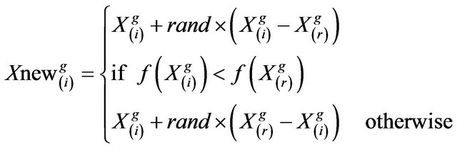(6)

2.4. Algorithm Termination

The algorithm is terminated after iterations are completed. Details of TLBO can be refereed in [1].

3. Proposed Weighted Teaching-LearningBased Optimizer (WTLBO)

Since the original TLBO is based on the principles of teaching-learning approach, we can always draw analogy with the real class room or learning scenario while designing TLBO algorithm. Although, a teacher always wishes that his/her student should achieve the knowledge equal to him in fast possible time but at times it becomes difficult for a student due to his/her forgetting characteristics. Teaching-learning process is an iterative process wherein the continuous interaction takes place for the transfer of knowledge. Every time a teacher interacts with a student he/she finds that the student is able to recall part of the lessons learnt from the last session. This is mainly due to the physiological phenomena of neurons in the brain. In this work we have considered this as our motivation to include a parameter known as “weight” in the Equations (4) and (6) of original TLBO. In contrast to the original TLBO, in our approach while computing the new learner value the part of its previous value is considered and that is decided by a weight factor w.

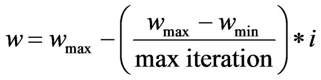
It is generally believed to be a good idea to encourage the individuals to sample diverse zones of the search space during the early stages of the search. During the later stages it is important to adjust the movements of trial solutions finely so that they can explore the interior of a relatively small space in which the suspected global optimum lies. To meet this objective we reduce the value of the weight factor linearly with time from a (predetermined) maximum to a (predetermined) minimum value:

(7)

where and are the maximum and minimum values of weight factor w, i iteration is the current iteration number and maxiteration is the maximum number of allowable iterations. and are selected to be 0.9 and 0.1, respectively.

Hence, in the teacher phase the new set of improved learners can be

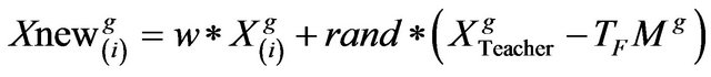(8)

and a set of improved learners in learner phase as

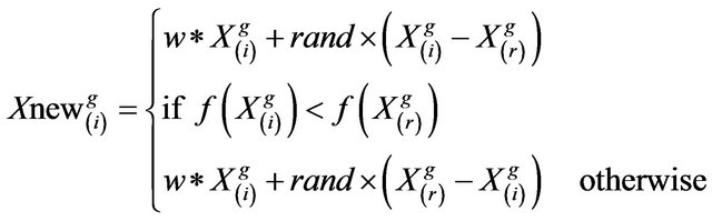(9)

4. Experimental Results

We have divided our experimental works into four sections. In Section 4.1, we have done performance comparison of WTLBO against basic algorithms like PSO, DE and TLBO to establish that our proposed approach performs better than above algorithms for investigated problems. We used 20 benchmark problems in order to test the performance of the PSO, DE, TLBO and the WTLBO algorithms. This set is large enough to include many different kinds of problems such as unimodal, multimodal, regular, irregular, separable, non-separable and multidimensional. For experiments in section 4.2 to Section 4.4 few functions from these 20 functions are used and those are mentioned in the comparison tables in respective sections of the paper. Initial range, formulation, characteristics and the dimensions of these problems are listed in Table 1.

In Section 4.2 of our experiments, attempts are made to compare our proposed approach with the recent variants of PSO as per [22,23]. The results of these variants are directly taken from [22,23] and compared with WTLBO. In Section 4.3, the performance comparisons are made with the recent variants of DE as per [22]. The Section 4.4 of our experiments devote to the performance comparison of WTLBO with Artificial Bee Colony (ABC) variants as in [24-27]. Readers may be intimated here that in all such above mentioned comparisons we have simulated WTLBO and basic PSO, DE and TLBO of our own but gained results of other algorithms directly from the referred papers.

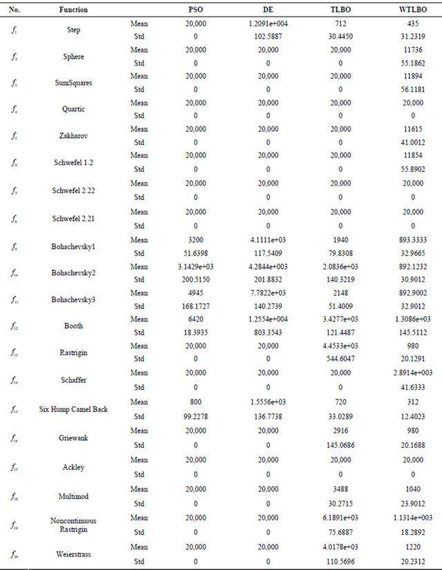
For comparing the speed of the algorithms, the first thing we require is a fair time measurement. The number of iterations or generations cannot be accepted as a time measure since the algorithms perform different amount of works in their inner loops, and they have different population sizes. Hence, we choose the number of fitness function evaluations (FEs) as a measure of computation time instead of generations or iterations. Since the algorithms are stochastic in nature, the results of two successive runs usually do not match. Hence, we have taken different independent runs (with different seeds of the random number generator) of each algorithm. Numbers of FEs for different algorithms which are compared with WTLBO are taken as in [22-27]. However, for WTLBO we have chosen 2.0 × 10⁴ as maximum number of FEs. The exact numbers of FEs in which we get optimal results with WTLBO are given in the Table 2.

Finally, we would like to point out that all the experiment codes are implemented in MATLAB. The experiments are conducted on a Pentium 4, 1 GB memory desktop in Windows XP 2002 environment

4.1. WTLBO vs PSO, DE and TLBO

In this Section, we have an exhaustive comparison of our proposed algorithm with various other evolutionary algorithms including basic TLBO. This section is divided into four sub sections, wherein we have compared WTLBO with various other algorithms. We have separately described the procedure in each sub section.

Parameter Settings

In all experiments in this section, the values of the common parameters used in each algorithm such as population size and total evaluation number were chosen to be the same. Population size was 20 and the maximum number fitness function evaluation was for all functions. The other specific parameters of algorithms are given below:

PSO Settings: Cognitive and social components, are constants that can be used to change the weighting beTable 1. List of benchmark functions have been used in experiment 1.

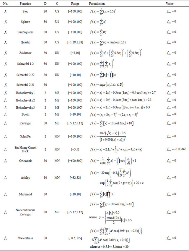
Table 2. No. of fitness evaluation comparisons of PSO, DE, TLBO, WTLBO (mean and standard deviation over 30 independent runs) after each algorithm was terminated after running for 20,000 FEs or when it reached the global minimum value before completely running for 20,000 FEs.

tween personal and population experience, respectively. In our experiments cognitive and social components were both set to 2. Inertia weight, which determines how the previous velocity of the particle influences the velocity in the next iteration, was 0.5.

DE Settings: In DE, F is a real constant which affects the differential variation between two Solutions and set to F = 0.5 * (1 + rand (0,1)) where rand (0,1) is a uniformly distributed random number within the range [0,1] in our experiments. Value of crossover rate, which controls the change of the diversity of the population, was chosen to be R = (Rmax – Rmin) * (MAXIT–iter)/MAXIT where Rmax = 1 and Rmin = 0.5 are the maximum and minimum values of scale factor R, iter is the current iteration number and MAXIT is the maximum number of allowable iterations as recommended in [28].

TLBO Settings: For TLBO there is no such constant to set.

WTLBO Settings: For WTLBO and are assigned as 0.9 and 0.1 respectively.

In Section 4.1, we compared the PSO, DE, TLBO and WTLBO algorithms on a large set of functions described in the previous section and are listed in Table 1. Each of the experiments in this section was repeated 30 times and it was terminated when it reached the maximum number of evaluations or when it reached the global minimum value with different random seeds and mean value and standard deviations of fitness value produced by the algorithms have been recorded in the Table 3 and at the same time mean value and standard deviations of No. of fitness evaluation produced by the algorithms have been recorded in the Table 2.

In order to analyze the results whether there is significance between the results of each algorithm, we performed t-test on pairs of algorithms which is quite popular among researchers in evolutionary computing [29]. In the Table 4 we report the statistical significance level of difference of the means of PSO and WTLBO algorithm, DE and WTLBO algorithm, TLBO and WTLBO algorithm. The t value is significant at a 0.05 level of significance by two tailed test. In table “+” indicates the t value is significant, and “NA” stands for Not applicable, covering cases for which the two algorithms achieve the same accuracy results.

From the Table 4, we get that in 15 cases WTLBO is significant then PSO, where as in 14 cases WTLBO is significant than DE, in 8 cases WTLBO is significant than TLBO.

4.2. WTLBO vs OEA, HPSO-TVAC, CLPSO and APSO

The experiments in this section constitute the comparison of the WTLBO algorithm versus OEA, HPSO-TVAC, CLPSO and APSO on 8 benchmarks described in [22], where OEA uses the number of FEs and HPSO-TVAC, CLPSO and APSO use the number of FEs, where as WTLBO runs for 2.0 × 10⁴ FEs. The results of OEA, HPSO-TVAC, CLPSO and APSO are gained from [22] and [23] directly. In the last column of Table 5 shows the significance level between best and second best algorithm using t test at a 0.05 level of significance by two tailed test. Note that here “+” indicates the t value is significant, and “NA” stands for Not applicable, covering cases for which the two algorithms achieve the same accuracy results. As can be seen from Table 5, WTLBO greatly outperforms OEA, HPSO-TVAC, CLPSO and APSO with better mean and standard deviation and numbers of FEs (refer Table 2 for WTLBO).

4.3. Experiment 3: WTLBO vs IADE, jDE and SaDE

The experiments in this section constitute the comparison of the WTLBO algorithm versus SaDE, jDE, JADE on 8 benchmark functions which are describe in [22]. The results of JADE, jDE and SaDE are gained from [22] directly. In the last column of Table 6 shows the significance level between best and second best algorithm using t test at a 0.05 level of significance by two tailed test. Note that here “+” indicates the t value is significant, and “NA” stands for Not applicable, covering cases for which the two algorithms achieve the same accuracy results It can be seen from Table 6 that WTLBO performs much better than these DE variants on almost all the functions.

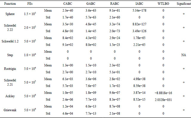
4.4. WTLBO vs CABC, GABC, RABC and IABC

The experiments in this section constitute the comparison of the WTLBO algorithm versus CABC [24], GABC [25], RABC [26] and IABC [27] on 8 benchmark functions. The parameters of the algorithms are identical to [26]. In the last column of Table 7 shows the significance level between best and second best algorithm using t test at a 0.05 level of significance by two tailed test. Note that here “+” indicates the t value is significant, and “NA” stands for Not applicable, covering cases for which the two algorithms achieve the same accuracy results The results, which have been summarized in Table 7, show that WTLBO performs much better in most cases than these ABC variants.

5. Conclusion and Further Research

In this paper an improved version of basic Teachinglearning based optimization (TLBO) technique is suggested and the performance of this compared with existing TLBO and other evolutionary computation techniTable 3. Performance comparisons of PSO, DE, TLBO, WTLBO in term of fitness value (mean and standard deviation over 30 independent runs) after each algorithm was terminated after running for 20,000 FEs or when it reached the global minimum value before completely running for 20,000 FEs.

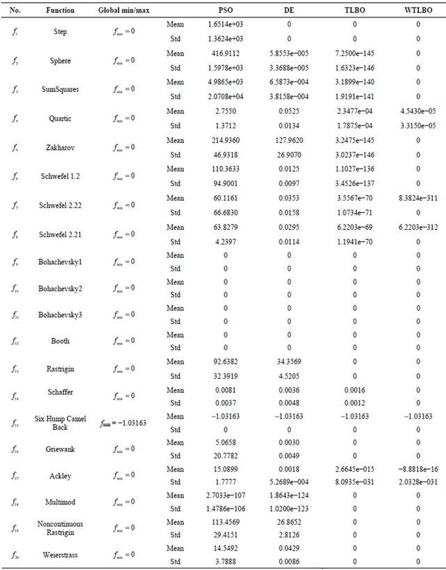
Table 4. t value, significant at a 0.05 level of significance by two tailed test using Table 3.

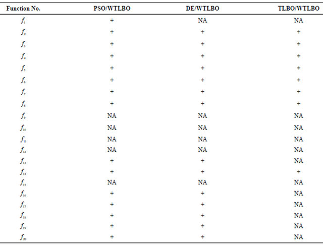
Table 5. Performance comparisons WTLBO, OEA, HPSO-TVAC, CLPSO and APSO in term of fitness value (mean and standard deviation over 30 independent runs) after OEA running of 3.0 × 10⁵ FEs, HPSO-TVAC, CLPSO and APSO use running 2.0 × 10⁵ FEs, and WTLBO running for 2.0 × 10⁴.

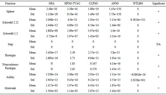
Table 6. Performance comparisons WTLBO, IADE, jDE and SaDE in term of fitness value (mean and standard deviation over 30 independent runs) after each algorithm was terminated after running by given FEs.

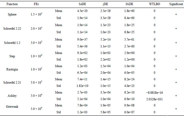
Table 7. Performance comparisons of WTLBO, CABC, GABC, RABC and IABC in term of fitness value (mean and standard deviation over 30 independent runs) after each algorithm was terminated after running by given FEs.

ques like PSO, DE, ABC and its variants. The proposed approach, known as Weighted-TLBO (WTLBO) is based on the natural phenomena of human brain (a learner’s brain) in forgetting the lessons learnt in last session. The paper suggested an inclusion of a parameter known as “weight” to address this phenomenon while using the learning equation in teaching and learning phases of basic TLBO algorithm. Although, inclusion of a parameter such as weight might seem to increase the complexity of the basic TLBO algorithm while tuning the parameter, the suggested approach in our work in setting up the weight parameter eases the task and able to provide better results compared to basic TLBO and all other investigated algorithms in this work for several benchmark functions. Our proposed WTLBO not only able to find global optima results but also does in faster computation time. This fact is verified from the number of function evaluations for WTLBO in each case from the results shown in our paper.

As a further research, we need to verify how this approach behaves with many other benchmark functions and some real world problems in data clustering.

REFERENCES

- R. V. Rao, V. J. Savsani and D. P. Vakharia, “Teaching- Learning-Based Optimization: A Novel Method for Constrained Mechanical Design Optimization Problems,” Computer-Aided Design, Vol. 43, No. 1, 2011, pp. 303- 315. doi:10.1016/j.cad.2010.12.015
- R. V. Rao, V. J. Savsani and D. P. Vakharia, “Teaching-Learning-Based Optimization: An Optimization Method for Continuous Non-Linear Large Scale Problems,” INS 9211 No. of Pages 15, Model 3G 26 August 2011.
- R. V. Rao, V. J. Savsani and J. Balic, “Teaching Learning Based Optimization Algorithm for Constrained and Unconstrained Real Parameter Optimization Problems,” Engineering Optimization, Vol. 44, No. 12, 2012, pp. 1447- 1462. doi:10.1080/0305215X.2011.652103
- R. V. Rao and V. K. Patel, “Multi-Objective Optimization of Combined Brayton and Inverse Brayton Cycles Using Advanced Optimization Algorithms,” Engineering Optimization, Vol. 44, No. 8, 2012, pp. 965-983. doi:10.1080/0305215X.2011.624183
- R. V. Rao and V. J. Savsani, “Mechanical Design Optimization Using Advanced Optimization Techniques,” Springer-Verlag, London, 2012. doi:10.1007/978-1-4471-2748-2
- V. Toğan, “Design of Planar Steel Frames Using Teaching-Learning Based Optimization,” Engineering Structures, Vol. 34, 2012, pp. 225-232. doi:10.1016/j.engstruct.2011.08.035
- R. V. Rao and V. D. Kalyankar, “Parameter Optimization of Machining Processes Using a New Optimization Algorithm,” Materials and Manufacturing Processes, Vol. 27, No. 9, 2011, pp. 978-985. doi:10.1080/10426914.2011.602792
- S. C. Satapathy and A. Naik, “Data Clustering Based on Teaching-Learning-Based Optimization. Swarm, Evolutionary, and Memetic Computing,” Lecture Notes in Computer Science, Vol. 7077, 2011, pp. 148-156, doi:10.1007/978-3-642-27242-4_18
- J. H. Holland, “Adaptation in Natural and Artificial Systems,” University of Michigan Press, Ann Arbor, 1975.
- J. G. Digalakis and K. G. Margaritis, “An Experimental Study of Benchmarking Functions for Genetic Algorithms,” International Journal of Computer Mathematics, Vol. 79, No. 4, 2002, pp. 403-416. doi:10.1080/00207160210939
- R. C. Eberhart and Y. Shi, “Particle Swarm Optimization: Developments, Applications and Resources,” IEEE Proceedings of International Conference on Evolutionary Computation, Vol. 1, 2001, pp. 81-86.
- R. C. Eberhart and Y. Shi, “Comparing Inertia Weights and Constriction Factors in Particle Swarm Optimization,” IEEE Proceedings of International Congress on Evolutionary Computation, Vol. 1, 2000, pp. 84-88.
- J. Kennedy and R. Eberhart, “Particle Swarm Optimization,” IEEE Proceedings of International Conference on Neural Networks, Vol. 4, 1995, pp. 1942-1948. doi:10.1109/ICNN.1995.488968
- J. Kennedy, “Stereotyping: Improving Particle Swarm Performance with Cluster Analysis,” IEEE Proceedings of International Congress on Evolutionary Computation, Vol. 2, 2000, pp. 303-308.
- Y. Shi and R. C. Eberhart, “Comparison between Genetic Algorithm and Particle Swarm Optimization,” Lecture Notes in Computer Science—Evolutionary Programming VII, Vol. 1447, 1998, pp. 611-616.
- Y. Shi and R. C. Eberhart, “Parameter Selection in Particle Swarm Optimization,” Lecture Notes in Computer Science Evolutionary Programming VII, Vol. 1447, 1998, pp. 591-600. doi:10.1007/BFb0040810
- Y. Shi and R. C. Eberhart, “Empirical Study of Particle Swarm Optimization,” IEEE Proceedings of International Conference on Evolutionary Computation, Vol. 3, 1999, pp. 101-106.
- R. Storn and K. Price, “Differential Evolution—A Simple and Efficient Heuristic for Global Optimization over Continuous Spaces,” Journal of Global Optimization, Vol. 11, No. 4, 1997, pp. 341-359. doi:10.1023/A:1008202821328
- R. Storn and K. Price, “Differential Evolution—A Simple and Efficient Adaptive Scheme for Global Optimization over Continuous Spaces,” Technical Report, International Computer Science Institute, Berkley, 1995.
- K. Price, R. Storn and A. Lampinen, “Differential Evolution a Practical Approach to Global Optimization,” Springer Natural Computing Series, Springer, Heidelberg, 2005.
- S. Das, A. Konar and U. K. Chakraborty, “Two Improved Differential Evolution Schemes for Faster Global Search,” Genetic and Evolutionary Computation Conference, Washington DC, 25-29 June 2005.
- Z. H. Zhan, J. Zhang, Y. Li and S. H. Chung, “Adaptive Particle Swarm Optimization,” IEEE Transactions on Systems, Man, and Cybernetics—Part B, Vol. 39, No. 6, 2009, pp. 1362-1381. doi:10.1109/TSMCB.2009.2015956
- A. Ratnaweera, S. Halgamuge and H. Watson, “Self-Organizing Hierarchical Particle Swarm Optimizer with Time-Varying Acceleration Coefficients,” IEEE Transactions on Evolutionary Computation, Vol. 8, No. 3, 2004, pp. 240- 255. doi:10.1109/TEVC.2004.826071
- B. Alatas, “Chaotic Bee Colony Algorithms for Global Numerical Optimization,” Expert Systems with Applications, Vol. 37, No. 8, 2010, pp. 5682-5687. doi:10.1016/j.eswa.2010.02.042
- G. P. Zhu and S. Kwong, “Gbest-Guided Artificial Bee Colony Algorithm for Numerical Function Optimization,” Applied Mathematics and Computation, Vol. 217, No. 7, 2010, pp. 3166-3173. doi:10.1016/j.amc.2010.08.049
- F. Kang, J. J. Li and Z. Y. Ma, “Rosenbrock Artificial Bee Colony Algorithm for Accurate Global Optimization of Numerical Functions,” Information Sciences, Vol. 181, No. 16, 2011, pp. 3508-3531. doi:10.1016/j.ins.2011.04.024
- W. F. Gao and S. Y. Liu, “Improved Artificial Bee Colony Algorithm for Global Optimization,” Information Processing Letters, Vol. 111, No. 17, 2011, pp. 871-882. doi:10.1016/j.ipl.2011.06.002
- S. Das and A. Abraham and A. Konar, “Automatic Clustering Using an Improved Differential Evolution Algorithm,” IEEE Transactions on Systems, Man, and Cybernetics—Part A: Systems and Humans, Vol. 38, No. 1, 2008.
- S. Das, A. Abraham, U. K. Chakraborty and A. Konar, “Differential Evolution Using a Neighborhood-Based Mutation Operator,” IEEE Transactions on Evolutionary Computation, Vol. 13, No. 3, 2009, pp. 526-553. doi:10.1109/TEVC.2008.2009457