Applied Mathematics
Vol.4 No.1(2013), Article ID:27089,5 pages DOI:10.4236/am.2013.41002
A New Iterative Scheme for Solving the Semi Sylvester Equation
Department of Mathematics, Persian Gulf University, Bushehr, Iran
Email: karimi@pgu.ac.ir, fatemehattarzadeh66@yahoo.com
Received October 20, 2012; revised November 20, 2012; accepted November 27, 2012
Keywords: Iterative Method; Multiple Linear Systems; Galerkin Projection Method;  -GL-LSQR Algorithm
ABSTRACT
In this paper, the Galerkin projection method is used for solving the semi Sylvester equation. Firstly the semi Sylvester equation is reduced to the multiple linear systems. To apply the Galerkin projection method, some propositions are presented. The presented scheme is compared with the  -GL-LSQR algorithm in point of view CPU-time and iteration number. Finally, some numerical experiments are presented to show that the efficiency of the new scheme.
1. Introduction
We want to solve, using Galerkin projection method, the following semi Sylvester equation
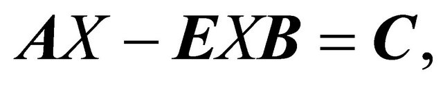 (1)
(1)
where A, E, B and C are![]() ,
, ![]() ,
, ![]() and
and ![]() matrices, respectively, and the unknown matrix
matrices, respectively, and the unknown matrix  is
is ![]() . Equation (1) has a unique solution if and only if
. Equation (1) has a unique solution if and only if  and
and  are regular matrix pairs with disjoint spectra, which will be assumed throughout this paper.
The semi Sylvester equations appear frequently in many areas of applied mathematics. We refer the reader to the elegant survey by Bhatia and Rosenthal [1] and references therein for a history of the equation and many interesting and important theoretical results. The semi Sylvester equations are important in a number of applications such as matrix eigen-decompositions [2,3], control theory [4,5], model reduction [6-8], numerical solution of matrix differential Riccati equations, and many more.
When the sizes of the coefficient matrices A and B are small, the popular and widely used numerical method is the Hessenberg-Schur algorithm [9]. For large and sparse matrices A and B, iterative schemes to solve the semi Sylvester equations such as those based on the matrix sign function or the Newton method are widely used [10-12]. During the last years, several projection methods based on Krylov subspace methods have also been proposed, see, e.g., [13-15] and the references therein. The main idea developed in these methods is to construct suitable bases of the Krylov subspace and projects the large problem into a smaller one. Naturally, a direct method such the one developed in [16] is used to solve the projected problem. The final step in the projection process consists in recovering the solution of the original problem from the solution of the smaller problem.
The semi Sylvesters Equation (1), in the special case, can be reduced to the following multiple linear systeam
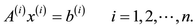 (2)
(2)
In [17], Ton F. Chan and Michael K. Ng presented the Galerkin projection method for solving linear systems (2). In this paper, we convert the semi Sylvester Equation (1) to the multiple linear system. We present some propositions for applying the Galerkin projection method to solve the reduced semi Sylvester equation. For showing the efficiency of the new scheme, in point of view CPUtime and iteration number, we compare the new scheme with the  -GL-LSQR algorithm [18]. Note that the semi Sylvester Equation (1) is converted to standard Sylvester equation, when E be a identity matrix I.
The remainder of the paper is organized as follows. Section 2 is devoted to a short review of the Galerkin projection method. In Section 3, we show that how to apply the Galerkin projection method for solving the semi Sylvester Equation (1). Some numerical experiments and comparing the new scheme with the  -GLLSQR algorithm, is devoted in Section 4. Finally, we make some concluding remarks in Section 5.
2. The Short Summary of Galerkin Projection Method
In this section, we consider using conjugate gradient (CG) methods for solving multiple linear systems  , for
, for , where the coefficient matrices
  and the right-hand side
  are different in general. In particular, we focus on the seed projection method which generates a Krylov subspace from a set of direction vectors obtained by solving one of the systems, called the seed system, by the CG method and then projects the residuals of other systems onto the generated Krylov subspace to get the approximate solutions. The whole process is repeated until all the systems are solved. CG methods can be seen as iterative solution methods to solve a linear system of equations by minimizing an associated quadratic functional. For simplicity, we let
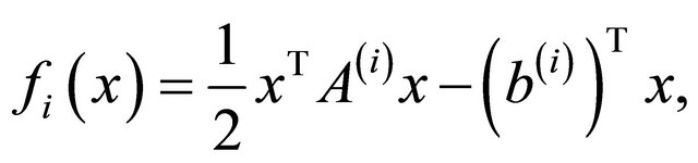 (3)
(3)
be the associated quadratic functional of the linear system . The minimizer of
  is the solution of the linear system
 . The idea of the projection method is that for each restart, a seed system
  is selected from the unsolved ones which are then solved by the CG method. An approximate solution
  of the nonseed system
  can be obtained by using search direction
  generated from the ith iteration of the seed system. More precisely, given the ith iterate
  of the nonseed system and the direction vector
 , the approximate solution
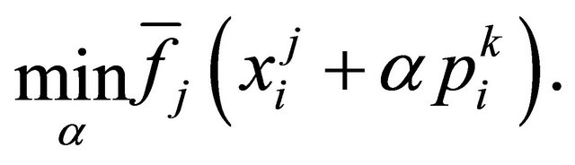
  is found by solving the following minimization problem
 (4)
(4)
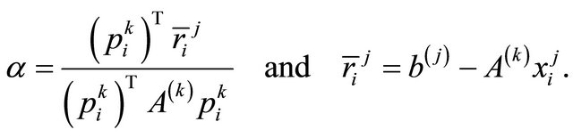
It is easy to check that the minimizer of (4) is attained at
 (5)
(5)
where
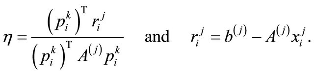 (6)
(6)
After the seed system  is solved to the desired accuracy, a new seed system is selected and the whole procedure is repeated. We note from (6) that the matrix-vector multiplication
  is required for each projection of the nonseed iteration. In general, the matrix-vector multiplication
 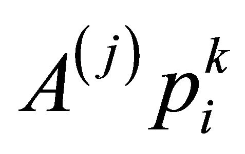 cannot be computed cheaply. The cost of the method will be expensive in the general case where the matrices
  and
and  are different.
In order to reduce the extra cost in projection method in the general case, we propose using the modified quadratic function ,
,
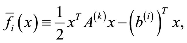
to compute the approximate solution of the nonseed system. Note that we have used  instead of
  in the above definition. In this case, we determine the next iterate of the nonseed system by solving the following minimization problem:
 (7)
(7)
The approximate solution  of the nonseed system
 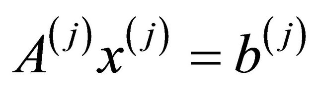 is given by
 (8)
(8)
where
 (9)
(9)
Now the projection process does not require the matrix-vector product involving the coefficient matrix  of the nonseed system. Therefore, the method does not increase the dominant cost (matrix-vector multiplies) of each CG iteration. Of course, unless
  is close to
  in some sense, we do not expect this method to work well because
  is then far from the current
 . So we have the following algorithm.
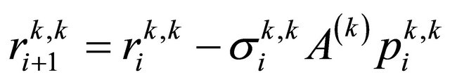
Algorithm 1 [17]: Preconditioned version of Projection Method
1. Set for  until all the systems are solved 2. Select the kth system as seed.
3. For  CG iteration,
4. For  unsolved systems 5. If
  then perform usual CG steps 6.
7. 
8. 
9. 
10. 
11. 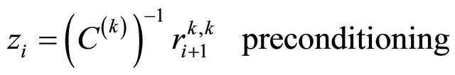
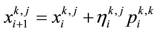
12. Else perform Galerkin projection 13. 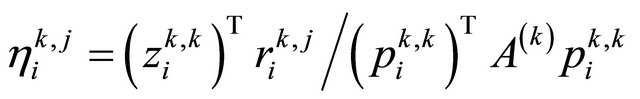
14. 
15. 
16. end if 17. end for 18. end for 19. end for
3. Solving the Semi Sylvester Equation
In this section, we focus on numerical solution of the semi Sylvester equations
 (10)
(10)
where ,
,  ,
,  ,
,  and
and  is the solution matrix. The semi Sylvester equation (10) has a unique solution if and only if
  and
and  are regular matrix pairs with disjoint spectra.
Now we want to apply Galerkin projection methods for solving the semi Sylvester Equation (10). Let B be symmetric matrix then semi Sylvester Equation (10) can be reduced to the following multiple linear systeams
 (11)
(11)
where ,
,  and
and .
.
By using the Schur decomposition, there is a unitary matrix  such that
 (12)
(12)
where  is diagonal matrix and it’s digonal components are the eigenvalues of
 . By substitution of (12) in (10), we have
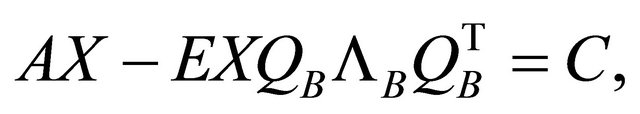
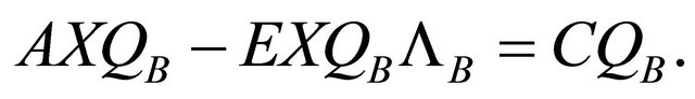
By taking  and
and , we obtain the following multiple linear systems
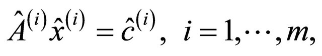 (13)
(13)
where ,
,  and
and  are
are , i-th column of the matrix
  and
and  -th column of the matrix
 , respectively.
To use the Galerkin projection method for solving the multiple linear systeams (13), it is need the matrix  to be symmetric positive definite. So the following propositons are presented and their proof are clear.
Proposition 1: Let A and B are symmetric matrices and E is symmetric positive definite matrix and
where  be the eigenvalues of matrix
 . Then
  is symmetric positive difinite.
Proposition 2: Let A, B and E be symmetric positive difinite matrices and symmetric positive semi-difinite matrix, respectively. Then  are symmetric positive definite, where
  be the eigenvalues of matrix
 .
.
Note that the semi Sylvester Equation (1) is converted to standard Sylvester equation, when E be a identity matrix I. Now by using the assumptions of the above propositions, we can apply the previous algorithm to solve the semi Sylvester Equation (10).
4. Numerical Experiments
In this section, all the numerical experiments were computed in double precision with some MATLAB codes. For all the examples the initial guess  was taken to be zero matrix. We apply the new scheme for solving the standard Sylvester equation.
For obtaining the numerical solution of the Sylvester equation by using new scheme, we consider two examples. At the first example the dense coefficient matrix is as the form
where  is an
is an ![]() matrix of uniformly distributed random integers and
matrix of uniformly distributed random integers and  is an identity matrix. At the second example the coeffient matrix is
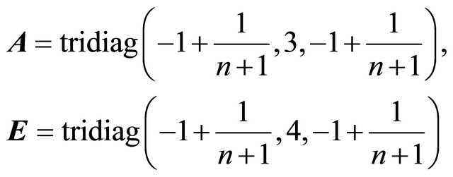
where  is
is  tridiagonal matrix. In both examples the matrix B is symmetric tridiagonal matrix with s size, as follows
Also the right-hand side matrix C in both examples is normalized random matrix. The  -GL-LSQR algorithm and Galerkin projection method are stopped when the residual norms of the first and second examples are less than 10−7 and 10−6, respectively.
In Table 1, we compare two  -GL-LSQR algorithm and Galerkin projection method for the first test example. We show that Galerkin projection method is better than
  -GL-LSQR algorithm in point of view CPU-time and iteration number. In this table, (s)m is the sum of iterations when we apply the Galerkin projection method for solving s linear systems (2). In Table 2, we compare the
  -GL-LSQR algorithm and Galerkin projection method for the second test example. We find that the
  -GL-LSQR algorithm is better in point of veiw the iteration number and the new scheme is better in point of veiw the CPU-time. Finally, Figures 1 and 2 show that the efficientcy of the Galerkin projection method for solving the semi Sylvester equation. In both tables, the symbols cond and iter are the condition number of the coefficient matrix A and the iteration number of the methods, respectively.
5. Conclusion
We proposed a new scheme for solving the semi Syl-
Table 1. Numerical results of the new scheme and  -GLLSQR algorithm for the semi Sylvester equation with the first example.
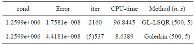
Table 2. Numerical results of the new scheme and  -GLLSQR algorithm for the semi Sylvester equation with the second example.
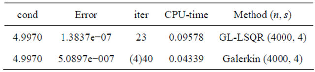
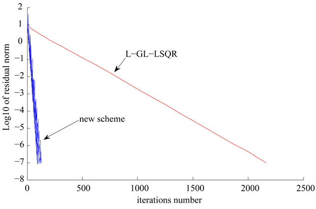
Figure 1. Comparing the new scheme with the  -GLLSQR algorithm with n = 500, s = 5.
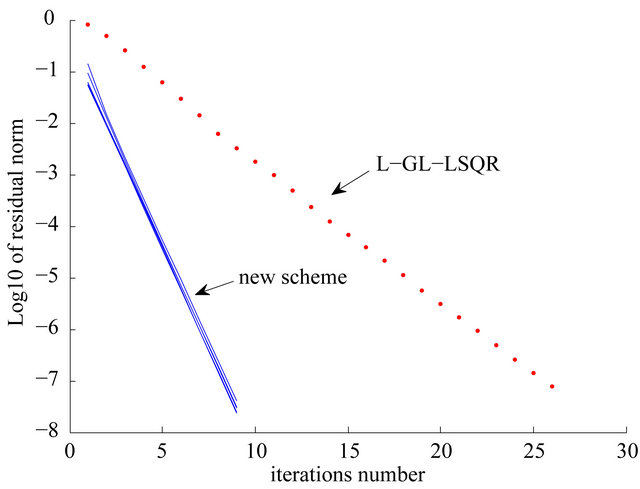
Figure 2. Comparing the new scheme with the  -GLLSQR algorithm with n = 4000 s = 4.
vester equation. By forcing some conditions on coefficent matrices A, B and E, We converted the semi Sylvester equation to s linear systems with different coefficent matrices and right-hands. Then we applied the Galerkin projection method for obtaining the numerrical solution, and we showed the efficiency of the new scheme. In Table 1, was shown that when the condition number of the coefficient matrix A is to be large then the new scheme is better then the  -GL-LSQR algorithm for solving the semi Sylvester equation. But in Table 2, the
  -GL-LSQR algorithm is better than new scheme in point of view iteration number for sparse and wellconditioned matrix A.
6. Acknowledgements
The authors would like to thank the anonymouws referees for their helpful suggestions, which would greatly improve the article.
REFERENCES
- R. Bhatia and P. Rosenthal, “How and Why to Solve the Operator Equation AX − XB = Y,” Bulletin London Mathematical Society, Vol. 29, No. 1, 1997, pp. 1-21. doi:10.1112/S0024609396001828
- G. H. Golub and C. F. Van Loan, “Matrix Computations,” 3rd Edition, Johns Hopkins University Press, Baltimore, 1996.
- V. Sima, “Algorithms for Linear-Quadratic Optimization,” Vol. 200, Pure and Applied Mathematics, Marcel Dekker, Inc., New York, 1996.
- B. Datta, “Numerical Methods for Linear Control Systems,” Elsevier Academic Press, New York, 2004.
- A. Lu and E. Wachspress, “Solution of Lyapunov Equations by ADI Iteration,” Computers & Mathematics with Applications, Vol. 21, 1991, pp. 43-58. doi:10.1016/0898-1221(91)90124-M
- A. C. Antoulas, “Approximation of Large-Scale Dynamical Systems,” Advances in Design and Control, SIAM, Philadelphia, 2005.
- U. Baur and P. Benner, “Cross-Gramian Based Model Reduction for Data-Sparse Systems,” Technical Report, Fakultat fur Mathematik, TU Chemnitz, Chemnitz, 2007.
- D. Sorensen and A. Antoulas, “The Sylvester Equation and Approximate Balanced Reduction,” Linear Algebra and Its Applications, Vol. 351-352, 2002, pp. 671-700. doi:10.1016/S0024-3795(02)00283-5
- G. H. Golub, S. Nash and C. Van Loan, “A Hessenberg Schur Method for the Problem AX + XB = C,” IEEE Transactions on Automatic Control, Vol. 24, No. 6, 1979, pp. 909-913. doi:10.1109/TAC.1979.1102170
- P. Benner, “Factorized Solution of Sylvester Equations with Applications in Control,” In: B. De Moor, B. Motmans, J. Willems, P. Van Dooren and V. Blondel, Eds., Proceedings of the 16th International Symposium on Mathematical Theory of Network and Systems, Leuven, 5-9 July 2004.
- W. D. Hoskins, D. S. Meek and D. J. Walton, “The Numerical Solution of the Matrix Equation XA + AY = F,” BIT, Vol. 17, 1977, pp. 184-190.
- D. Y. Hu and L. Reichel, “Application of ADI Iterative Methods to the Restoration of Noisy Images,” Linear Algebra and Its Applications, Vol. 172, No. 15, 1992, pp. 283-313. doi:10.1016/0024-3795(92)90031-5
- A. El Guennouni, K. Jbilou and A. J. Riquet, “Block Krylov Subspace Methods for Solving Large Sylvester Equations,” Numerical Algorithms, Vol. 29, No. 1, 2002, pp. 75-96. doi:10.1023/A:1014807923223
- K. Jbilou, “Low Rank Approximate Solutions to Large Sylvester Matrix Equations,” Applied Mathematics and Computation, Vol. 177, No. 1, 2006, pp. 365-376. doi:10.1016/j.amc.2005.11.014
- M. Robb and M. Sadkane, “Use of Near-Breakdowns in the Block Arnoldi Method for Solving Large Sylvester Equations,” Applied Numerical Mathematics, Vol. 58, No. 4, 2008, pp. 486-498. doi:10.1016/j.apnum.2007.01.025
- G. H. Golub, S. Nash and C. Van Loan, “A Hessenberg Schur Method for the Problem AX + XB = C,” IEEE Transactions on Automatic Control, No. 24, No. 6, 1979, pp. 909-913.
- T. Chan and M. Ng, “Galerkin Projection Methods for Solving Multiple Linear Systems,” Department of Mathematics, University of California, Los Angeles, 1996.
- S. Karimi, “A New Iterative Solution Method for Solving Multiple Linear Systeams,” Advances in Linear Algebra and Matrix Theory, Vol. 1, 2012, pp. 25-30. doi:10.4236/alamt.2012.23004