Applied Mathematics
Vol.3 No.11A(2012), Article ID:24753,13 pages DOI:10.4236/am.2012.331241
On the Detection of Visual Features from Digital Curves Using a Metaheuristic Approach
Department of Mathematics and Computer Science, University of Cagliari, Cagliari, Italy
Email: dirubert@unica.it
Received May 28, 2012; revised June 27, 2012; accepted July 5, 2012
Keywords: Digital Curve; Dominant Point; Polygonal Approximation; Ant Colony Optimization
ABSTRACT
In computational shape analysis a crucial step consists in extracting meaningful features from digital curves. Dominant points are those points with curvature extreme on the curve that can suitably describe the curve both for visual perception and for recognition. Many approaches have been developed for detecting dominant points. In this paper we present a novel method that combines the dominant point detection and the ant colony optimization search. The method is inspired by the ant colony search (ACS) suggested by Yin in [1] but it results in a much more efficient and effective approximation algorithm. The excellent results have been compared both to works using an optimal search approach and to works based on exact approximation strategy.
1. Introduction
Computer imaging has developed as an interdisciplinary research field whose focus is on the acquisition and processing of visual information by computer and has been widely used in object recognition, image matching, target tracking, industrial dimensional inspection, monitoring tasks, etc. Among all aspects underlying visual information, the shape of the objects plays a special role. In computational shape analysis an important step is representation of the shape in a form suitable for storage and/or analysis. Due to their semantically rich nature, contours are one of the most commonly used shape descriptors, and various methods for representing the contours of 2D objects have been proposed, each achieves, more or less successfully, the most desirable features of a proper representation, such as data compression, simplicity of coding and decoding, scaling and invariance under rigid motions, etc. After shape representation, another crucial step in shape analysis consists in extracting meaningful features from digital curves. Attneave [2] pointed out that information on a curve is concentrated at the dominant points. Dominant points are those points that have curvature extreme on the curve and they can suitably describe the curve for both visual perception and recognition. Following Attneave’s observation, there are many approaches developed for detecting dominant points. They can be classified into two main categories: corner detection approaches and polygonal approximation approaches. The phrases dominant point detection and poly gonal approximation are used alternatively by some researchers in the area of pattern recognition. The polygonnal approximation methods in fact construct polygon by connecting the detected dominant points. Although dominant points can constitute an approximating polygon, the polygonal approximation is different from the dominant point detection in concept. The polygonal approximation seeks to find a polygon that best fits the given digital curve. It can be applied to produce a simplified representation for storage purposes or further processing. Corner detection approaches aim to detect potential significant points, but they cannot represent smooth curve appropriately. For dominant point-detection approaches, Teh and Chin [3] determined the region of support for each point based on its local property to evaluate the curvature. The dominant points are then detected by a nonmaxima suppression process. Wu and Wang [4] proposed the curvature-based polygonal approximation for dominant point detection. It combines the corner detection and polygonal approximation methods, and it can detect the dominant points effectively. Wang et al. [5] proposed a simple method that uses the directions of the forward and backward vectors to find the bending value as the curvature. Held et al. [6] proposed a two-stage method. In the first stage, a coarse-to-fine smoothing scheme is applied to detect dominant points. Then, in the second stage, a hierarchical approximation is produced by a criterion of perceptual significance. Carmona et al. [7] proposed a new method for corner detection. A normalized measurement is used to compute the estimated curvature and to detect dominant points, and an optimization procedure is proposed to eliminate collinear points. The performance of most dominant point-detection methods depends on the accuracy of the curvature evaluation. For polygonal approximation approaches, sequential, iterative, and optimal algorithms are commonly used. For sequential approaches, Sklansky and Gonzales [8] proposed a scan-along procedure which starts from a point and tries to find the longest line segments sequentially. Ray and Ray [9] proposed a method which determines the longest possible line segments with the minimum possible error. Most of the sequential approaches are simple and fast, but the quality of their approximating results depends on the location of the point where they start the scan-along process and, as a consequence, they can miss important features. The family of iterative approaches splits and merges curves iteratively until they meet the preset allowances. For split-and-merge approaches, Ramer [10] estimated the distances from the points to the line segments of two ending points. The segment is partitioned at the point with the maximum distance until the maximum distance is not greater than an allowable value. Ansari and Delp [11] proposed another technique which first uses Gaussian smoothing to smooth the boundary and then takes the maximal curvature points as break points to which the split-and-merge process is applied. Ray and Ray [12] proposed an orientation-invariant and scale-invariant method by introducing the use of ranks of points and the normalized distances. If a poor initial segmentation is used, the approximation results of the split-and-merge approaches maybe far from the optimal one. The iterative approaches, in fact, suffer the sensitivity to the selection of the starting points for partitioning curves. The optimal approaches tend to find the optimal polygonal approximation based on specified criteria and error bound constraints. The idea behind is to approximate a given curve by an optimal polygon with the minimal number of line segments such that the approximation error between the original curve and the corresponding line segments is no more than a pre-specified tolerance [1]. All of the local optimal methods are very fast but their results maybe very far from the optimal one. Unfortunately, an exhaustive search for the vertices of the optimal polygon from the given set of data points results in an exponential complexity. Dunham [13] and Sato [14] used dynamic programming to find the optimal approximating polygon. But, when the starting point is not specified, the method requires a worst-case complexity of O(n4) where n is the number of data points. Fortunately, there exist some global search heuristics which can find solutions very close to the global optimal one in a relative short time. Approaches based on genetic algorithms [15,16] and tabu search [17] have been proposed to solve the polygonal approximation problem and they obtain better results than most of the local optimal methods. Sun and Huang [15] presented a genetic algorithm for polygonal approximation. An optimal solution of dominant points can be found. However, it seems to be time consuming. Yin [17] focused in the computation efforts and proposed the tabu search technique to reduce the computational cost and memory in the polygonal approximation. Horng [18] proposed a dynamic programming approach to improve the fitting quality of polygonal approximation by combining the dominant point detection and the dynamic programming. Generally, the quality of the approximation result depends upon the initial condition where the heuristics take place and the metric used to measure the curvature. To solve complex combinatorial optimization problems metaheuristic techniques have been introduced. Fred Glover [19] first coined the term metaheuristic as a strategy that guides another heuristic to search beyond the local optimality such that the search will not get trapped in local optima. Metaheuristic techniques combine two components, an exploration strategy and an exploitation heuristic, in a framework. The exploration strategy searches for new regions, and once it finds a good region the exploitation heuristic further intensifies the search for this area. In this context, metaheuristics encompass several wellknown approaches such as genetic algorithm (GA), simulated annealing, tabu search (TS), scatter search, ant colony optimization and particle swarm optimization. Most of the central metaheuristic methods have been applied to the polygonal approximation problems and attained promising results.
In this paper we present a method that combines the dominant point detection and the ant colony optimization search. The method is inspired by the ant colony search suggested by Yin in [1] but it results in a much more efficient and effective approximation algorithm. The excellent results have been compared both to works using an optimal search approach and to works based on exact approximation strategy. The ant colony optimization framework is presented in Section 2. The proposed method for detecting dominant points is illustrated in Section 3. In Section 4 the proposed algorithm is applied both on real world curves and on four well-known benchmark curves. The performance is compared visually and numerically with many existing methods. Conclusions are presented in Section 5.
2. Ant Colony System Algorithms
In [20] Dorigo first proposed the Ant Colony System (ACS) algorithm as a computational scheme inspired by the way in which real ant colonies operate. Ants make use of a substance called pheromone to communicate information about the shortest paths to reach the food. An ant on the move leaves a certain amount of pheromone on the ground, creating a path formed by a trail of this substance. While an isolated ant moves practically at random, an ant encounters a trace left above. The ant is able to detect it and decide, most likely, to follow it, thus reinforcing the trail with its own pheromone. As a result, the more ants follow a trail, the more attractive the path becomes to follow and the probability with which an ant chooses a path increases with the number of ants that previously chose the same path (Figure 1 [21]).
The ACS scheme is inspired by this process. We apply it to the problem of the polygonal approximation. The method we propose is similar to that described by Yin in [1] but it solves the problem in a much more efficient and effective way. In the ACS algorithm artificial ants build solutions (tours) of a problem moving from one node of a graph to another. The algorithm performs  iterations. During each iteration m ants construct a tour by performing n steps in which it is applied a probabilistic decision rule (transition state). In practice, if an ant in node i chooses to move to node j, the edge
  is added to the tour in progress. This step is repeated until the ant has completed its tour. After all the ants have built their tours, each ant deposits some pheromone on the pheromone trail associated to the visited edges to make them most desirable for future ants. The amount of pheromone trail
  associated with edge
  represents the desirability of choosing node j from the node i and also represents the desirability that the edge
  belongs to the tour built by an ant. The pheromone trail information is changed during solution of the problem to reflect the experience acquired by ants during solving the problem. Ants deposit an amount of pheromone proportional to the quality of the solutions they produced: the shorter the tour generated by an ant, the greater the amount of pheromone deposited on the edge used to generate the tour. This choice supports research directed
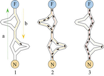
Figure 1. The first ant locates the food source (F), following one of the possible ways (a), then comes back to the nest (N), leaving behind a pheromone trail (b). Ants follow any way at random, but the reinforcement of the beaten path makes it more attractive as the shortest route. Ants take preferably this way while other paths lose their pheromone trails.
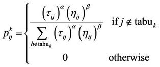
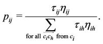
towards good solutions. A pheromone evaporation is introduced to avoid stagnation, that is the situation where all ants choose the same tour [22]. Each ant has memory of the nodes already visited. The memory (or internal state) of each ant, called tabu list, is used to define, for each ant k, the set of nodes that an ant lying on the node i, has yet to visit. Exploiting the memory then, an ant k can build feasible solutions by generating a graph of the state space. The probability that an ant k chooses to move from node i to node j is defined as:
 (1)
(1)
where  is the intensity of pheromone associated with edge
 ,
,  is the value of visibility of edge
 ,
,  and
and  are control parameters, and
  is the set of currently inaccessible nodes for the ant k according to the problem-domain constraints. The value of visibility is determined by a greedy heuristic for the initial problem, which considers only the local information on the edge
 , as its length. The role of the parameters
  and
and  is the following. If
 , closer nodes are more likely to be chosen: this corresponds to a classical stochastic greedy algorithm (with multiple starting points since ants are initially randomly distributed on the nodes). If, however,
  , the solution depends on the pheromone only: this case will lead to a rapid emergence of a stagnation situation with the corresponding generation of tours which are strongly sub-optimal. A trade-off between the heuristic value of track and intensity is therefore necessary.
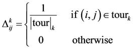
After all ants have completed their tour, each ant  deposits a quantity of pheromone
  on each edge which has used:
 (2)
(2)
where  is the tour done by ant
  at current cycle and
  is its length. The value
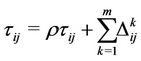
  depends on how well the ant has worked: the shorter the tour done, the greater the amount of pheromone deposited. At the end of every cycle, the intensity of traces of pheromone on each edge is updated by the pheromone updating rule:
 (3)
(3)
where  is the persistence rate of previous trails,
  is the amount of pheromone laid on edge
  by the ant
  at the current cycle, and
  is the number of ants.
ACS algorithms have been applied to several discrete optimization problems, such as the travelling salesman problem and the quadratic assignment problem. Recent applications cover problems like vehicle routing, sequential ordering, graph coloring, routing in communication networks, and so on. In this work we propose the scheme of ACS to solve the problem of the polygonal approximation.
3. The ACS-Based Proposed Method
In this section we describe how we use the ACS algorithm to solve the problem of polygonal approximation. We first define our problem in terms of discrete optimization problem and how we represent it in terms of a graph. Then, we illustrate the proposed method from the initialization phase to the searching and refining the optimal path.
3.1. Problem Formulation
Given a digital curve represented by a set of N clockwise-ordered points,  where
where  is considered as the succeeding point of
 , we define arc
  as the collection of those points between
  and
and , and chord
  as the line segment connecting
  and
and . In approximating the arc
  by the chord
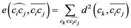
 , we make an error, denoted by
  that can be measured by any distance norm; for here, the
  norm, i.e., the sum of squared perpendicular distance from every data point on
  to
to , is adopted. Thus, we have
 (4)
(4)
where  is the perpendicular distance from point
  to the corresponding chord
 . The distance
  is measured as follows:
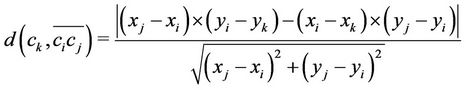 (5)
(5)
where  are the spatial coordinates of the points
 , respectively.
The objective is to approximate a given curve by an optimal polygon with the minimal number of line segments such that the approximation error between the original curve and the corresponding line segments is less than a pre-specified tolerance. Formally, the aim is to find the minimal ordered set  where
where  and
and , and the set of M line segments
 composes an approximating polygon to the point set C such that the error norm between C and P is no more than a pre-specified tolerance,
 . The error norm between C and P, denoted by
 , is then defined as the sum of the approximation errors between the M arcs
 and the corresponding M line segments
 :
:
 (6)
(6)
where  and
and  is the approximation error between the arc
  and the chord
 , as defined in (4).
3.2. Graph Representation
In order to apply the ACS algorithm, we need to represent our problem in terms of a graph, . For the polygonal approximation problem, each point on the curve should be represented as a node of the graph, i.e.,
  , where C is the set of points on the given curve. E is an ideal edge set that has the desired property that any closed circuit which originates and ends at the same node represents a feasible solution to the original problem, i.e., the approximating polygon consisting of the edges and nodes along the closed circuit should satisfy the
  - bound constraint,
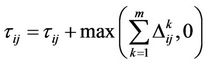
 . We construct the edge set by penalizing the intensity of pheromone trails on the paths to make them less attractive if they don’t satisfy the
  -bound constraint. The edge set E is thus generated as follows. Initially, the set E is created as an empty set. Then, new edges are added to it. For every node
 , we examine each of the remaining nodes,
  , in clockwise order. If the approximation error between the arc
  and the line segment
  is no more than
 , then the directed edge
  is added to the edge set E. Thus, we have:
 (7)
(7)
The edge is directed to avoid the ants walking backward. Then, the problem of polygonal approximation is equivalent to finding the shortest closed path on the directed graph  such that
 . In the following, the closed path completed by the ant k will be denoted by tourk, the number of nodes visited by the ant k in the tourk will be
  and the approximation error between the original curve C and the approximating polygon corresponding to tourk will be
 .
.
3.3. Starting Node Initialization and Selection
During each iteration each ant chooses a starting node in the graph and sequentially constructs a closed path to finish its tour. In order to find the shortest closed tour, it is convenient to place the ants at the nodes with a higher probability of finding such a tour, instead of a randomly distribution. For the selection of the starting nodes we propose two alternative strategies, we call Selection_1 and Selection_2. Let’s describe the two algorithms in detail.
Selection_1 algorithm
One of the most common shape descriptors is the shape signature (or centroidal profile) [23]. A signature is one-dimensional functional representation of boundary, obtained by computing the distance of the boundary from the centroid as a function of angle (a centroidal profile). This simple descriptor is useful to understand the complexity of a shape. The more the extrema (maxima and minima) of the signature, the more articulated the object is. The number of signature extrema and the boundary points corresponding to them help us both to determine automatically the number of distributed ants and to select the nodes on the graph they choose to start their tour. In this algorithm the number m of ants to distribute on the graph is equal to the number of the signature extrema. Also, the m boundary points correspondent to the extrema represent the m starting nodes at the beginning of the first cycle. If  is the list of the boundary points relative to the extrema of the signature, then the ant k starts its first tour from the node sk,
 . The signature extrema are localized in the boundary points near to the most concave or convex portions of the curve. In such portions the most significant points (i.e. dominant points) of the curve are located. This is the reason for choosing the signature extrema as starting nodes at the first cycle. In the next cycles, the ants are placed at the nodes with higher probability to find the shortest closed tour. We thus create a selection list for the starting nodes, denoted by
 . Initially,
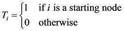 (8)
(8)
The probability with which the node  is chosen as a starting node in the next cycles, denoted
 , is estimated as the value
  normalized by the sum of all values,
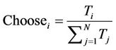 (9)
(9)
At the end of each cycle, the value of  is updated. Let’s denote by
  the set of ants which start with the node
  at the current cycle and by
  its size. We update the value
  making a trade-off between the average quality of current solutions constructed by the ants in
  and the value of
  derived from older cycles. Thus, we let
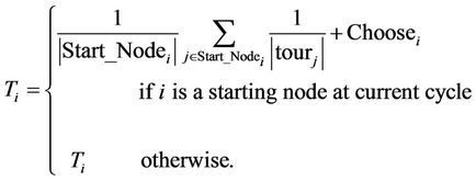 (10)
(10)
During the process, the ants will tend to choose the starting nodes which have more experiences of constructing shorter tours and enforce an exploitation search to the neighborhood of better solutions.
Selection_2 algorithm
For each node  of the graph we evaluate the greatest approximation error among all the directed edges departing from i. We thus generate a list of the N greatest approximation errors sorted in ascending order. We select the first D edges, where D is a percentage on N (in all the experiments
 ) and derive the nodes where these edges depart from. The list of such nodes, after eliminating duplications, represents the set of the starting nodes at the beginning of the first cycle and its size is the number m of the ants to distribute on the graph. As in the previous algorithm, we then create a selection list for the starting node
 , initialized as described in Equation (8). In the next iterations, the probability with which the node i is chosen as a starting node and the updating of the value
  are accomplished as in the previous strategy, according to the Equations (9) and (10).
3.4. Node Transition Rule
As described in Section 2, the probability with which an ant k chooses to move from node i to node j is determined by the pheromone intensity  and the visibility value
  of the corresponding edge. In the proposed method,
  is equally initialized to 1/N (actually, any small constant positive value may be fine), and is updated at the end of each cycle according to the average quality of the solutions that involve this edge. The value of
  is determined by a greedy heuristic which guides the ants to walk to the farthest accessible node in order to construct the longest possible line segment in a hope that an approximating polygon with fewer vertices is obtained eventually. This can be accomplished by setting
 , where
  is the number of points on
 . The value of
  is fixed during all the cycles since it considers local information only. The transition probability from node i to node j through directed edge
  is defined as
 (11)
(11)
3.5. Pheromone Updating Rule
At the end of each cycle we update the intensity of pheromone trails of an edge by the average quality of the solutions involving this edge by simply applying Equations (2) and (3). At the end of each cycle, the pheromone intensity at directed edge  is updated by
 (12)
(12)
where  is the quantity of new trails left by the ant k and it is computed by
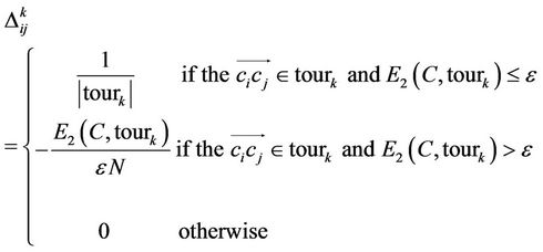 (13)
(13)
According to the ACS paradigm, more quantities of pheromone trails will be laid at the edges along which most ants have constructed shorter feasible tours. As a result, the proposed rule will guide the ants to explore better tours corresponding to high quality solutions.
3.6. Refinement of Approximation Polygon
Once dominant points have been detected we apply an enhancement process to refine the point localization according to a minimal distance criterion. Let
 the ordered set of detected dominant points. Considering the couples
  and
and ,
,  , the refinement process consists in moving the intermediate point
  between
  and
and  in a new point by a local minimization distance. For all the points
  in the arc
  we evaluate the sum of the approximation errors,
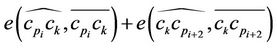 . The new position for the point
  is chosen as follows:
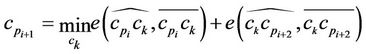 (14)
(14)
The new dominant point  between
  and
and  is then used in the rest of the process. The refinement step is repeated for each pair
 ,
, .
.
The refining phase terminates by deleting very close dominant points.
3.7. Summary of the Proposed Method
We summarize the proposed algorithm, denoted Poly_by_ ACS, as follows:
The Poly_by_ACS Algorithm
Input:
 : a set of clockwise ordered points.
N_max: the maximal number of running cycles.
1) Inizialization:
Construct the directed graph  as described in
Subsection 3.2.
Determine the number  of ants as described in
Subsection 3.3.
Set  for every directed edge
 .
.
Initialize  for
for  as described in
Subsection 3.3.
Set NC = 1, where NC is the cycle counter.
Set .
.
2) For every ant do
Select a starting node as described in Subsection
3.3.
Repeat
Move to next node according to the node
transition rule using Equation (11).
until a closed tour is completed.
3) Find out the shortest feasible tour, say current_tour among the m tours obtained in Step 2.
4) If  or
or
 and
and
then .
.
5) For every directed edge  do
do
Update the pheromone intensity using Equations (12) and (13).
6) For every selection entry  do
do
Update the entry value using Equation (8).
7) If (NC < N_max) NC = NC + 1 and go to Step 2;
8) Refine the approximation polygon as described in
Subsection 3.6.
4. Experimental Results and Comparisons
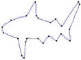
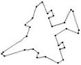
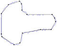
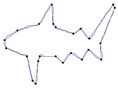
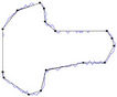
In this section we present the experimental results of the proposed ACS-based approximation algorithm. For all the processed curves we have tested both the two node selection strategies. From now on, we call Method_1 and Method_2 the approximation methods based on Selection_1 and Selection_2 algorithms, respectively. The two methods have been firstly tested on some real world images (fish, aircraft, hand, noisy key), showed in Figure 2. For each curve, the initial starting nodes, the polygonal approximation before and after refining the detected dominant points by applying Method_1 and Method_2 are showed in Figures 3-6. The performances of our algorithms have been compared to those of the method proposed by Yin [1]. The parameters used for Yin’s method have been chosen according to the suggestion of the author’s algorithm. In Table 1 we present the comparative performance evaluation between our methods and Yin’s one. For each image we have evaluated the initial number of points, N, the number of detected dominant points, Np, and the approximation error between the original curve and the corresponding optimal polygon, . For all the images, our methods show a much better efficacy in approximating real noisy world shapes, both before and after the refining step. In all cases we obtain a lower approximation error associated to a significant reduction of Np. Also, our algorithms are less parameters dependent than Yin’s one. Apart the
  -bound constraint and the number of the maximum cycles, Yin’s ACS method uses other five parameters. The goodness of the approximating polygon is strongly dependent on the chosen parameter values. Our methods
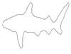

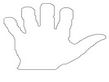
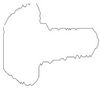
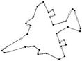
Figure 2. Some real world curves: fish, aircraft, hand and key.
 (a)
(a)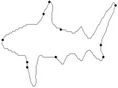 (b)
(b)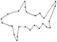 (c)
(c)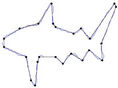 (d)
(d)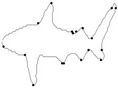 (e)
(e)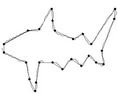 (f)
(f)
Figure 3. Fish contour: the initial starting nodes, the polygonal approximation before and after refining the detected dominant points by applying Method_1 in (a), (b), (c) and by applying Method_2 in (d), (e), (f), respectively.
 (a)
(a)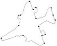 (b)
(b)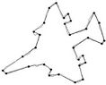 (c)
(c)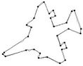 (d)
(d)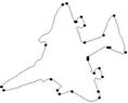 (e)
(e)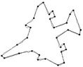 (f)
(f)
Figure 4. F10 contour: the initial starting nodes, the polygonal approximation before and after refining the detected dominant points by applying Method_1 in (a), (b), (c) and by applying Method_2 in (d), (e), (f), respectively.
 (a)
(a)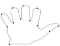 (b)
(b)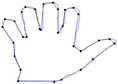 (c)
(c) (d)
(d)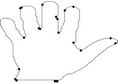 (e)
(e)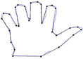 (f)
(f)
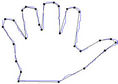
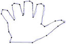
Figure 5. Hand contour: the initial starting nodes, the polygonal approximation before and after refining the detected dominant points by applying Method_1 in (a), (b), (c) and by applying Method_2 in (d), (e), (f), respectively.
 (a)
(a)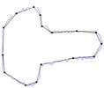 (b)
(b) (c)
(c)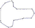 (d)
(d)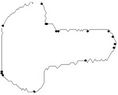 (e)
(e)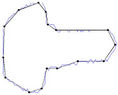 (f)
(f)
Figure 6. Key contour: the initial starting nodes, the polygonal approximation before and after refining the detected dominant points by applying Method_1 in (a), (b), (c) and by applying Method_2 in (d), (e), (f), respectively.
automatically choose the number of distributed ants and do not need any other parameter. We only define the maximum number of iterations and the  -bound. Moreover, since the approach is non deterministic, different runs can lead to different solutions. We have approached this problem by choosing the initial set of starting nodes automatically and by introducing a refinement step to reduce the approximation error. Such two aspects are not present in Yin’s approach. Finally, the approximation
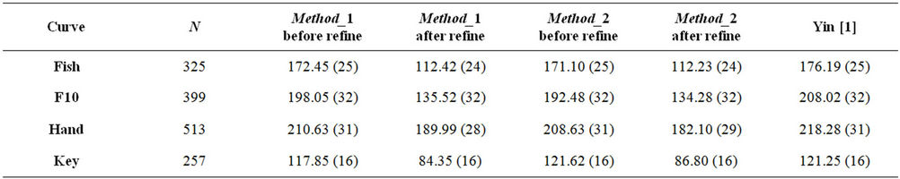
Table 1. The approximation error E2 for the real curves for our methods and Yin’s algorithm (in parentheses the number of dominant points).
error levels off after only few iterations of the iterative process (in case of F10 curve after 3 iterations we achieve the best value 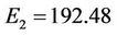 and in case of hand curve just one iteration is needed to get
 ). This means that our methods are computationally more efficient, too. The proposed algorithms have been, also, tested on four benchmark curves (leaf, chromosome, semicircle and infinite), commonly used in many previous approaches. The experimental results have been compared to many existing methods for dominant point detection. For each proposed approximation algorithm we show the number of detected point, Np, the approximation error,
  , the compression ratio,
  , the combinations of the compression ratio and the approximation error,
  ,
,  and
and , as suggested in [7] and [24]. The compression ratio and the approximation error are combined to measure the efficiency of the dominant point detectors and to compare them. The dominant points (circled) detected by our methods on benchmark curves (Figure 7) are showed in Figure 8 and the comparative results with other methods are presented in Table 2. The results can be summarized as follows:
• The number of dominant points detected by our approach is an average value of the number detected by other algorithms.
• The values of  and
and  are smaller than all the other algorithms, except Carmona [7] in processing chromosome curve and Horng [18] in processing semicircle curve.
• The values of  and
and  are smaller than the values supplied by other algorithms. In some cases they are a little bit greater than Marji-Siy [27] and Carmona [7] methods.
By analyzing the comparative results, we can affirm that the proposed approach is superior to many existing algorithms based on exact search methodology. To demonstrate the feasibility of our approach we have, also, compared it to other methods based on global search heuristic, like ACS_Poly method proposed in [1], the GA-based method proposed in [16] and the TS-based method proposed in [17]. The results presented in Table 3 confirm the superiority of our method both in effec-
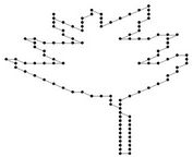
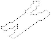

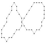
Figure 7. The benchmark curves: leaf, chromosome, semicircle, infinite.

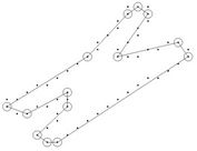
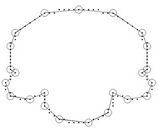
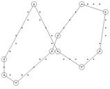
Figure 8. Dominant points (circled) for the benchmark curves.
tiveness (in terms of Np and ) and in efficiency (in terms of computational cost) since only few iterations are needed to localize the vertices of the approximating polygon. Finally, we have compared our approach to other methods in order to check how the refining step is able to improve the quality of the polygonal approximation. We have analyzed the four real world curves, fish, F10, hand and key. Each of them has been first processed by our methods, Method_1 and Method_2, by Yin’s one [1], by Teh-Chin’s one [3] and by Wu’s ones [26,28]. On each polygonal approximation we have then applied the refining procedure in order to get a better localization of dominant points and consequently a lower error,
 . As
. As

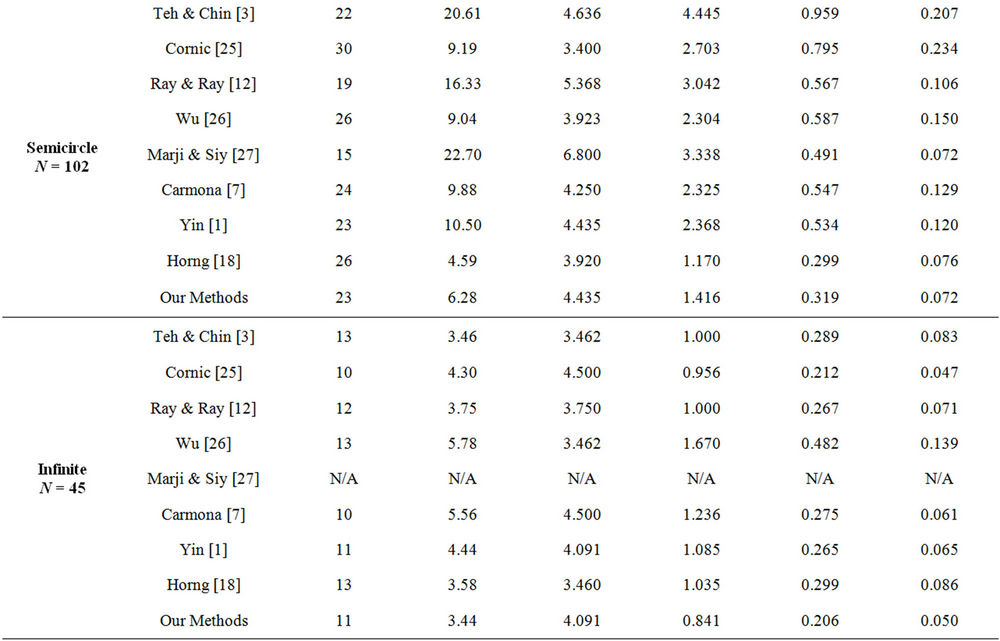
Table 2. Comparison with other methods on the benchmark curves.
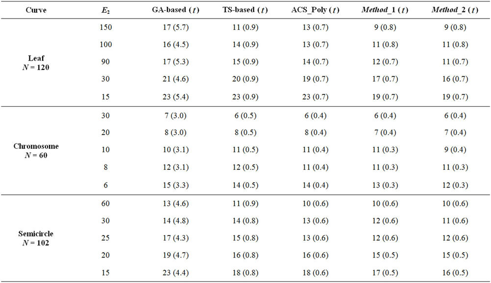
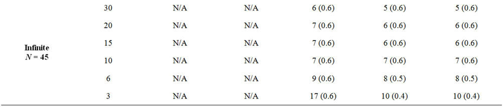
Table 3. Comparison in terms of approximation error, E2, number of dominant points, Np, and CPU time, t in seconds, on the benchmark curves.
we can see from the numerical results showed in Table 4, the refining procedure is able to improve all the polygonnal approximations. In all the cases we get a lower error, . However, the best approximations are still achieved by applying our method, confirming its superiority as a general approach for dominant point detection and polygonal approximation. Some visual comparisons are showed in Figures 9 and 10.
5. Conclusion
In this work we have presented a novel method for approximating a digital curve. The algorithm is inspired by the ant colony search suggested by Yin in [1] but it has resulted in a much more efficient and effective approximation algorithm. The performance of our approach has been first compared to that of the method proposed by Yin on some real world curves. The experimental results have showed a much better efficacy in approximating real noisy world shapes, both before and after the refining step. Also, our algorithms are less parameters dependent than Yin’s one. Apart the  -bound constraint and the number of the maximum cycles, Yin’s ACS method uses other five parameters and the goodness of the approximating polygon is strongly dependent on the chosen parameter values. On the contrary, our approach automatically choose the number of distributed ants. No other parameters are used in the whole process. Also, the localization of the best dominant points can be obtained by the refinement step in a very fast way. Finally, the performances of our methods level off after only few iterations of the approximating process. This means that our methods are computationally more efficient, too. We can summarize the differences and the contribution of our approach against the one in [1] in four main aspects: less parameter dependance, automatic choosing of starting points and number of distributed ants, updating of the best tour during search (Step 4 of the Poly_by_ACS Algorithm) and refining. First preliminary results of our

Table 4. Comparison with other methods, without or with the refinement step, on real world curves.
 (a)
(a)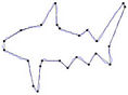 (b)
(b) (c)
(c)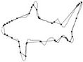 (d)
(d) (e)
(e)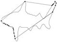 (f)
(f)
Figure 9. Visual comparisons with other methods on fish contour: (a) Method_1; (b) Method_2; (c) Yin’s [1], (d) TehChin’s [3], (e) Wu’s [28] and (f) Wu’s [26].
 (a)
(a)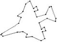 (b)
(b)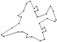 (c)
(c)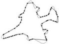 (d)
(d)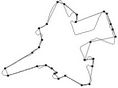 (e)
(e) (f)
(f)
Figure 10. Visual comparisons with other methods on F10 contour: (a) Method_1; (b) Method_2; (c) Yin’s [1]; (d) TehChin’s [3]; (e) Wu’s [28]; and (f) Wu’s [26].
approach have been presented in [29]. In the new version we have proposed in this paper we have introduced the possibility to delete very close dominant points, by obtaining a significant reducing of NP with a negligible in-
 (a)
(a)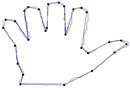 (b)
(b) (c)
(c)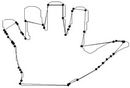 (d)
(d)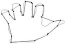 (e)
(e)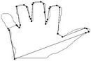 (f)
(f)
Figure 11. Visual comparisons with other methods on hand contour: (a) Method_1; (b) Method_2; (c) Yin’s [1]; (d) TehChin’s [3]; (e) Wu’s [28]; and (f) Wu’s [26].
 (a)
(a)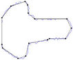 (b)
(b)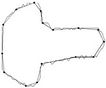 (c)
(c)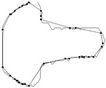 (d)
(d)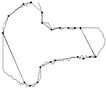 (e)
(e)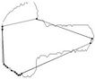 (f)
(f)
Figure 12. Visual comparisons with other methods on key contour: (a) Method_1; (b) Method_2; (c) Yin’s [1]; (d) TehChin’s [3]; (e) Wu’s [28]; and (f) Wu’s [26].
creasing of approximation error. We have expanded the experimental results by visual comparisons with other methods (Figures 9-12). Also, we have tested the importance and the effectiveness of refinement step, as showed in Table 4. The performance of our algorithms have been tested on four contour commonly used curves (leaf, chromosome, semicircle and infinite) in many previous approaches. This testing has confirmed that the proposed approach is superior to many existing algorithms based on exact search methodology. Finally, our approach has been compared to other methods based on global search heuristic, like ACS_Poly method proposed in [1], the GA-based method proposed in [16] and the TS-based method proposed in [17]. Again, the excellent results have confirmed the superiority of our methods both in effectiveness (in terms of Np and ) and in efficiency (in terms of computational cost). The two proposed algorithms, Method_1 and Method_2, have comparable performances, if applied on very simple curves, as we can see from the results shown in Table 2. However, if applied on real world curves, Method_2 presents a lower approximation error, both before and after the refining step, as we can see in Table 1. Finally, we can notice another little difference on behalf of Method_2 in Table 3, where we present the number of detected dominant points with a same approximation error.
REFERENCES
- P. Y. Yin, “Ant Colony Search Algorithms for Optimal Polygonal Approximation of Plane Curves,” Pattern Recognition, Vol. 36, No. 8, 2003, pp. 1783-1797. doi:10.1016/S0031-3203(02)00321-7
- E. Attneave, “Some Informational Aspects of Visual Percaption,” Psychological Review, Vol. 61, No. 3, 1954, pp. 183-193. doi:10.1037/h0054663
- C.-H. Teh and R. T. Chin, “On the Detection of Dominant Points on Digital Curves,” IEEE Transactions on Pattern Analysis and Machine Intelligence, Vol. 11, No. 8, 1989, pp. 859-871. doi:10.1109/34.31447
- W. Y. Wu and M. J. Wang, “Detecting the Dominant Points by the Curvature-Based Polygonal Approximation,” CVGIP: Graphical Model Image Processing, Vol. 55, No. 2, 1993, pp. 79-88. doi:10.1006/cgip.1993.1006
- M. J. Wang, W. Y. Wu, L. K. Huang and D. M. Wang, “Corner Detection Using Bending Value,” Pattern Recognition Letters, Vol. 16, No. 8, 1995, pp. 575-583. doi:10.1016/0167-8655(95)80003-C
- A. Held, K. Abe and C. Arcelli, “Towards a Hierarchical Contour Description via Dominant Point Detection,” IEEE Transactions on System Man Cybernetics, Vol. 24, No. 6, 1994, pp. 942-949. doi:10.1109/21.293514
- A. Carmona-Poyato, N. L. Fernández-Garca, R. MedinaCarnicer and F. J. Madrid-Cuevas, “Dominant Point Detection: A New Proposal,” Image and Vision Computing, Vol. 23, No. 13, 2005, pp. 1226-1236. doi:10.1016/j.imavis.2005.07.025
- J. Sklansky and V. Gonzalez, “Fast Polygonal Approximation of Digitized Curves,” Pattern Recognition, Vol. 12, No. 5, 1980, pp. 327-331. doi:10.1016/0031-3203(80)90031-X
- B. K. Ray and K. S. Ray, “Determination of Optimal Polygon from Digital Curve Using L1 Norm,” Pattern Recognition, Vol. 26, No. 4, 1993, pp. 505-509. doi:10.1016/0031-3203(93)90106-7
- U. Ramer, “An Iterative Procedure for the Polygonal Approximation of Plane Curves,” Computer Graphics Image Processing, Vol. 1, No. 3, 1972, pp. 244-256. doi:10.1016/S0146-664X(72)80017-0
- N. Ansari and E. J. Delp, “On Detecting Dominant Points,” Pattern Recognition, Vol. 24, No. 5, 1991, pp. 441-450. doi:10.1016/0031-3203(91)90057-C
- B. K. Ray and K. S. Ray, “A New Split-and-Merge Technique for Polygonal Approximation of Chain Coded Curves,” Pattern Recognition Letters, Vol. 16, No. 2, 1995, pp. 161-169. doi:10.1016/0167-8655(94)00081-D
- J. G. Dunham, “Optimum Uniform Piecewise Linear Approximation of Planar Curves,” IEEE Transactions on Pattern Analysis and Machine Intelligence, Vol. 8, No. 1, 1986, pp. 67-75. doi:10.1109/TPAMI.1986.4767753
- Y. Sato, “Piecewise Linear Approximation of Plane Curves by Perimeter Optimization,” Pattern Recognition, Vol. 25, No. 12, 1992, pp. 1535-1543. doi:10.1016/0031-3203(92)90126-4
- S. C. Huang and Y. N. Sun, “Polygonal Approximation Using Genetic Algorithms,” Pattern Recognition, Vol. 32, No. 8, 1999, pp. 1409-1420. doi:10.1016/S0031-3203(98)00173-3
- P. Y. Yin, “Genetic Algorithms for Polygonal Approximation of Digital Curves,” International Journal of Pattern Recognition and Artificial Intelligence, Vol. 13, No. 7, 1999, pp. 1-22. doi:10.1142/S0218001499000598
- P. Y. Yin, “A Tabu Search Approach to the Polygonal Approximation of Digital Curves,” International Journal of Pattern Recognition and Artificial Intelligence, Vol. 14, No. 2, 2000, pp. 243-255. doi:10.1142/S0218001400000167
- J. H. Horng, “Improving Fitting Quality of Polygonal Approximation by Using the Dynamic Programming Technique,” Pattern Recognition Letters, Vol. 23, No. 14, 2002, pp. 1657-1673. doi:10.1016/S0167-8655(02)00129-0
- F. Glover, “Future Paths for Integer Programming and Links to Artificial Intelligence,” Computers & Operations Research, Vol. 13, No. 5, 1986, pp. 533-549. doi:10.1016/0305-0548(86)90048-1
- M. Dorigo, “Optimization, Learning, and Natural Algorithms,” Ph.D. Thesis, Politecnico di Milano, Milano, 1992.
- Wikipedia, 2012. http://en.wikipedia.org/wiki/Ant_colony_optimization
- M. Dorigo, G. Di Caro and L. M. Gambardella, “Ant Algorithms for Discrete Optimization,” Artificial Life, Vol. 5, No. 2, 1999, pp.137-172. doi:10.1162/106454699568728
- L. Costa and R. Cesar, “Shape Analysis and Classification Theory and Practice,” CRC Press, Boca Raton, 2001.
- P. Y. Yin, “Polygonal Approximation of Digital Curves Using the State-of-the-Art Metaheuristics,” In: G. Obinata and A. Dutta, Eds., Vision Systems: Segmentation and Pattern Recognition, I-Tech, Vienna, 2007, pp. 451-464. doi:10.5772/4974
- P. Cornic, “Another Look at Dominant Point Detection of Digital Curves,” Pattern Recognition Letters, Vol. 18, No. 1, 1997, pp. 13-25. doi:10.1016/S0167-8655(96)00116-X
- W. Y. Wu, “Dominant Point Detection Using Adaptive Bending Value,” Image and Vision Computing, Vol. 21, No. 6, 2003, pp. 517-525. doi:10.1016/S0262-8856(03)00031-3
- M. Marji and P. Siy, “A New Algorithm for Dominant Points Detection and Polygonization of Digital Curves,” Pattern Recognition, Vol. 36, No. 10, 2003, pp. 2239- 2251. doi:10.1016/S0031-3203(03)00119-5
- W. Y. Wu, “A Dynamic Method for Dominant Point Detection,” Graphical Models, Vol. 64, No. 5, 2003, pp. 304-315. doi:10.1016/S1077-3169(02)00008-4
- C. Di Ruberto and A. Morgera, “A New Algorithm for Polygonal Approximation Based on Ant Colony System,” Lecture Notes in Computer Science, Vol. 5716, 2009, pp. 633-641. doi:10.1007/978-3-642-04146-4_68