Applied Mathematics
Vol.5 No.6(2014), Article ID:44491,10 pages DOI:10.4236/am.2014.56081
Application of the Homotopy Perturbation Method to Nonlinear Heat Conduction and Fractional Van der Pol Damped Nonlinear Oscillator
T. A. Nofel
Mathematics Department, Faculty of Science, Taif University, Taif, Saudi Arabia
Email: nofal_ta@yahoo.com
Copyright © 2014 by author and Scientific Research Publishing Inc.
This work is licensed under the Creative Commons Attribution International License (CC BY).
http://creativecommons.org/licenses/by/4.0/


Received 7 December 2013; revised 7 January 2014; accepted 14 January 2014
ABSTRACT
In this paper, a powerful analytical method, called He’s homotopy perturbation method is applied to obtaining the approximate periodic solutions for some nonlinear differential equations in mathematical physics via Van der Pol damped non-linear oscillators and heat transfer. Illustrative examples reveal that this method is very effective and convenient for solving nonlinear differential equations. Comparison of the obtained results with those of the exact solution, reveals that homotopy perturbation method leads to accurate solutions.
Keywords:Nonlinear Oscillators, Homotopy Perturbation Method, Fractional Van der Pol Damped Nonlinear Oscillator, Heat Transfer

1. Introduction
In recent years, the application of the homotopy perturbation method in non-linear problems has been developed by scientists and engineers, because this method continuously deforms the difficult problem under study into a simple problem which is easier to solve. The homotopy perturbation method was proposed first by He in 1998 [1] and was developed and improved by He [2] -[5] . Homotopy, is an important part of differential topology. Actually the homotopy perturbation method is a coupling of the traditional perturbation method and the homotopy method in topology [6] . The study of nonlinear problems is of crucial importance not only in all areas of physics but also in engineering and other disciplines, since most phenomena in our world are essentially nonlinear and are described by nonlinear equations. It is very difficult to solve nonlinear problems and, in general, it is often more difficult to get an analytic approximation than a numerical one for a given nonlinear problem.
Recently, several methods have been used to find approximate solutions to nonlinear problems, such as, the homotopy perturbation method [2] -[7] , the variational iteration method [8] -[10] , and the energy balance method [11] -[14] .
In this paper, we present a new application of He’s homotopy perturbation method. The paper is organized as follows: In Section 2, we present a brief summary about the homotopy perturbation method. Some applications are then discussed in Section 3. A comparison between the analytical solution obtained and numerical solution by Runge-Kutta method has been discussed and displayed graphically in Section 4. Finally, conclusions are drawn in Section 5.
Variation, which ; is called a correct function. The solution of the linear problems can be solved in a single iteration step due to the exact identification of the Lagrange multiplier. The principles of the variational iteration method and its applicability for various kinds of differential equations are given in [8] [15] -[19] . In this method, it is required first to determine the Lagrange multiplier
  optimally. The successive approximation
 of the solution u will be readily obtained upon using the determined Lagrange multiplier and any selective function
 , consequently, the solution is given by
 .
.
2. Basic Idea of He’s Homotopy Perturbation Method
The homotopy pertirabation method is one of the important methods to find the approximate solutions for nonlinear partial differential equations in mathematical physics. The homotopy perturbation method, which was originally proposed by J. H. He [2] -[5] in 1999, has been proved by many authors to be a powerful mathematical tool for solving various kinds of problems [2] -[5] . This method introduces an efficient approach for a wide variety of scientific and enginering applications. We should point out that this method can give the approximte or exact solutions without the computation of the Adomian polynomial, discretization, linearization, transformation or perturbation. To illustrate, consider the following nonlinear differential equation [2] -[5] :
 (1)
(1)
with the boundary conditions of the following form:
 (2)
(2)
where  is a general differential operator,
  a boundary operator,
  a known analytical function and
  the boundary of the domain
 . Generally speaking, the operator
  can be divided into two parts which are
  and
and , where
  is linear, but
  is nonlinear . Equation (1) can therefore be rewritten as follows :
 (3)
(3)
By the homotopy technique, we construct a homotopy  which satisfies
 (4)
(4)
 (5)
(5)
where  is an embedding parameter,
  is an initial approximation of Equation (1), which satisfies the boundary conditions (2). Obviously, from Equations (4) and (5) we have
 (6)
(6)
 (7)
(7)
The changing process of  from zero to unity is just that of
  from
from  to
to  In Topology, this is called deformation, and
  and
and  are called homotopy. According to the homotopy perturbation method, we can first use the embedding parameter “p” as a small parameter, and assume that the solution of Equations (4) and (5) can be written as a power series in “p” as follows:
 (8)
(8)
On setting  results in the approximate solution of Equation (3), we have:
 (9)
(9)
The combination of the perturbation method and the homotopy method is called the homotopy perturbation method. This method has eliminated the limitations of the traditional perturbation methods, while keeping their advantages. The series (9) is convergent in most cases. However, the convergence rate depends on the nonlinear operator  (the following opinions are suggested by He [2] -[5] ):
1) The second derivative of  with respect to
  must be small because the parameter may be relatively large, i.e.,
2) The norm of  must be smaller than 1 so that the series converges.
Consequently, the construction of the homotopy plays an important role in solving a nonlinear problem with He’s homotopy perturbation method, and therefore is problem dependent.
3. Applications
In order to assess the accuracy of the homotopy perturbation method (HPM) for solving nonlinear equations and to compare the solution it gives with the exact solution, we will consider the following examples.
3.1. Example 1: Classical Fractional Van der Pol Oscillator
The classical fractional Van der Pol damped nonlinear oscillator can be represented by the following nonlinear equation [14] [15]
 (10)
(10)
Rewrite Equation (10) in the following form
 (11)
(11)
From Equation (11), one can establish the following homotopy
 (12)
(12)
where  is an imbedding parameter. As in He’s homotopy perturbation method [2] -[4] , it is obvious that when
 , Equation (12) becomes a linear differential equation for which an exact solution can be calculated; for
 , Equation (12) then becomes the original problem. Now the homotopy parameter
  is used to expand the solution
  as follows:
 (13)
(13)
Setting  leads to the approximate solution of the problem:
 (14)
(14)
Substituting Equation (13) into Equation (12) and equating the terms with the identical powers of 
 (15)
(15)
 (16)
(16)
Solving Equation (15), we have [16]
 (17)
(17)
The Fourier series for  has been calculated and is given by [17] .
 (18)
(18)
where ,
, 
Substituiting from Equations (17) and (18) into Equation (16), we get
 (19)
(19)
Eliminating the secular term, we get
 (20)
(20)
From the above equation, we can easily find that
 (21)
(21)
which is the same with that obtained by the iteration procedure (see Equation (40) in [14] and Equation (23) in [15] ). Hence, the approximate periodic solution takes the form:
 (22)
(22)
To illustrate and verify the accuracy of this method, we may compare the approximate periodic solution  and the exact periodic solution. The exact solution
  for the classical fractional Van der Pol damped nonlinear oscillator is as follows [18] :
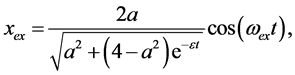 (23)
(23)
where
 (24)
(24)
We make a comparasion between the exact solution (23) and the approximate solution (22) when ,
,  as shown in Table 1.
In Figure 1 we present a variety of comparisons between the approximate and exact solution for Equation (10). For ,
, . It can be observed that Equation (22) provides an excellent approximation to the exact periodic solution in Equation (23).
From Figure 1 and Table 1, the approximate solutions have the same behavior as the exact solution so that the approximate solutions is rapidly convergent to the exact solution.
3.2. Example 2: Rayleigh Equation
The special case of the fractional Van der Pol damped nonlinear oscillator [19] or the Rayleigh equation [20] can be represented by

Table 1. Comparison between the approximate solution (22) and the exact solution (23) for Equation (17).
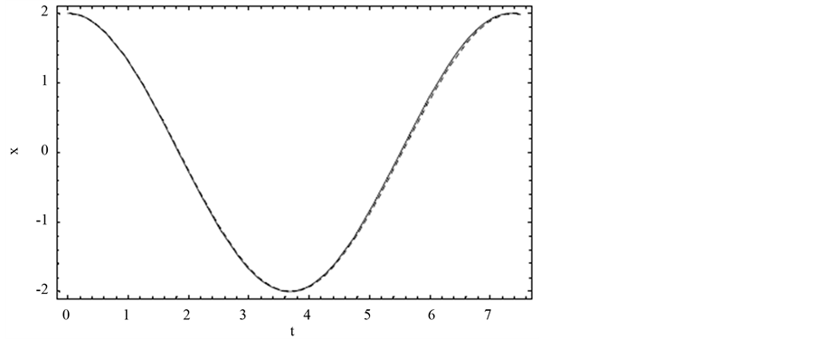
Figure 1. Comparison of the approximate periodic solution with the exact solution for an initial condition of  and
and  in Example 1.
 (25)
(25)
Equation (25) can be written in the form
 (26)
(26)
Therefore, we can establish the following homotopy
 (27)
(27)
Proceeding in the same way as example 1, substituting from Equation (13) into Equation (27) and equating the terms with the identical powers of 
 (28)
(28)
 (29)
(29)
The solution for  is given by
 (30)
(30)
Substituting from Equation (30) into Equation (29) we have
 (31)
(31)
Eliminating the secular terms, we obtain
 (32)
(32)
From the above equation, we can easily find that
 (33)
(33)
Hence, the approximate periodic solution can be readily obtained:
 (34)
(34)
To write the exact periodic solution  we used its values from [17] , and for approximate values we used Equation (34). In fact the exact periodic solution can be obtained from the following complicated relation, as given in [18]
 (35)
(35)
where
 (36)
(36)
We now draw a comparasion between the exact and approximate solutions when ,
,  as shown in Table 2.
Figure 2 shows the comparison between the approximate periodic solution  obtained from formula (34) and the exact periodic solution
  obtained from formula (35) see [18] . It is shown that the approximate periodic solution is nearly identical with that given by the exact periodic solution.
From Figure 2 and Table 2, the approximate solution has the same behavior as the exact solution so that the approximate solution is rapidly convergent to the exact solution.
Table 2. Comparison between the approximate and exact solutions for Equation (25). For ,
, .
.
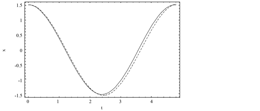
Figure 2. Comparison of the approximate periodic solution with the exact solution for an initial condition of  and
and  in Example 2.
3.3. Example 3: Cooling of a Lumped System by Combined Convection and Radiation
Most scientific problems such as heat transfer are inherently nonlinear. We know that except for a limited number of problems, most of the problems do not have an analytical solution. Therefore, these nonlinear equations should be solved using other methods. Some of them are solved using numerical techniques and some are solved using the analytical method of perturbation. In this example we will consider the problem of combined convective-radiative cooling of a lumped system [21] . Let the system have volume , surface area
 , density
 , specific heat
 , emissivity
  and the initial temperature
 . At
. At , the system is exposed to an environment with convective heat transfer with the coefficient of
  and the temperature
 . The system also loses heat through radiation and the effective sink temperature is
 . The cooling equation and the initial conditions are as follows:
 (37)
(37)
 (38)
(38)
To solve Equation (37), we introduce the following changes of parameters:
 (39)
(39)
After parameter change, the heat transfer equation will result in the following:
 (40)
(40)
 (41)
(41)
For simplicity, we assume the case . So we have
 (42)
(42)
 (43)
(43)
For Equation (42) we can establish the following homotopy
 (44)
(44)
 (45)
(45)
Proceeding as before. The homotopy parameter  is used to expand the solution
  as follow
 (46)
(46)
Setting  leads to the approximate solution of the problem:
 (47)
(47)
By the homotopy perturbation method, we can obtain a series of linear equations, and we write only the first three linear equations by substituting Equation (46) into Equation (40) and equating the terms with the identical powers of 
 (48)
(48)
 (49)
(49)
 (50)
(50)
Consequently, solving the above equations, the first few components of the homotopy perturbation solution for (48)-(50) are derived as follows:
 (51)
(51)
 (52)
(52)
 (53)
(53)
So  will generally equal when
  the following expression:
 (54)
(54)
The exact solution of Equation  is obtained by Aziz [21] in the following form:
 (55)
(55)
We make a comparison between the exact and approximate solutions when  as shown in Table 3.
Applying the Runge-Kutta technique, the numerical solution of Equation (42) is calculated and plotted in Figure 3. The difference between the analytical and numerical results is negligible.
Table 3. Comparison between the approximate and exact solutions for Equation (16) when .
.
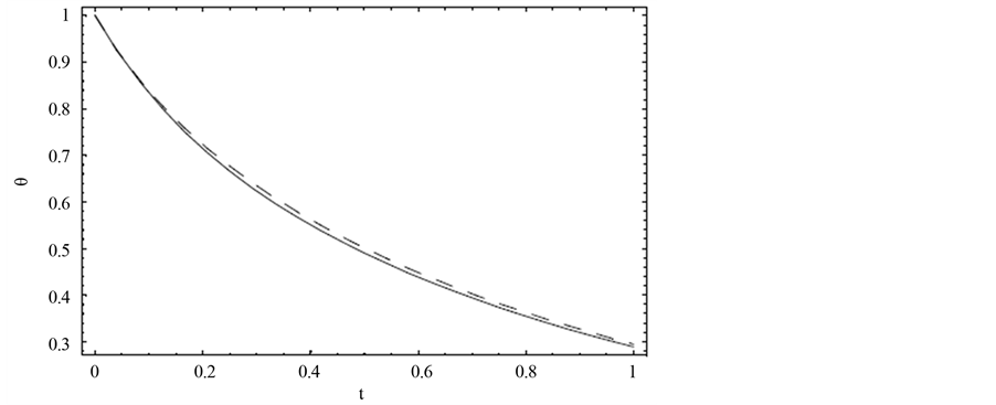
Figure 3. Comparison of the approximate periodic solution with the exact solution for  in Example 3.
From Figure 3 and Table 3 the approximate solution has the same behavior as the exact solution so that the approximate solution is rapidly convergent to the exact solution.
4. Conclusion
In this paper, the homotopy perturbation method has been successfully used to study nonlinear oscillator problems. He’s homotopy perturbation method which is proved to be a powerful mathematical tool for the study of nonlinear oscillators, can be easily extended to any nonlinear oscillator problem. The solutions obtained are in good agreement with exact values. Finally, we have found out that the homotopy perturbation method leads to more acceptable results even for large .
.
References
- He, J.H. (1999) Homotopy Perturbation Technique. Computer Methods in Applied Mechanics and Engineering, 178, 257-262. http://dx.doi.org/10.1016/S0045-7825(99)00018-3
- He, J.H. (2006) New Interpretation of Homotopy Perturbation Method. International Journal of Modern Physics B, 20, 2561-2568. http://dx.doi.org/10.1142/S0217979206034819
- He, J.H. (1999) Homotopy Perturbation Technique. Computer Methods in Applied Mechanics and Engineering, 178, 257-262. http://dx.doi.org/10.1016/S0045-7825(99)00018-3
- He, J.H. (2000) A Coupling Method of Homotopy Technique and Perturbation Technique for Nonlinear Problems. International Journal of Non-Linear Mechanics, 35, 37-43. http://dx.doi.org/10.1016/S0020-7462(98)00085-7
- He, J.H. (2006) Some Asymptotic Methods for Strongly Nonlinear Equations. International Journal of Modern Physics B, 20, 1141-1199. http://dx.doi.org/10.1142/S0217979206033796
- He, J.H. (2000) New Perturbation Technique Which Is Also Valid for Large Parameters. Journal of Sound and Vibration, 229, 1257-1263. http://dx.doi.org/10.1006/jsvi.1999.2509
- Shou, D.H. (2009) THE Homotopy Perturbation Method for Nonlinear Oscillators. Computers & Mathematics with Applications, 58, 2456-2459. http://dx.doi.org/10.1016/j.camwa.2009.03.034
- He, J.H. (2007) Variational Iteration Method—Some Recent Results and New Interpretations. Journal of Computational and Applied Mathematics, 207, 3-17. http://dx.doi.org/10.1016/j.cam.2006.07.009
- He, J.H. and Wu, X.H. (2006) Construction of Solitary Solution and Compacton-Like Solution by Variational Iteration Method. Chaos Solitons & Fractals, 29, 108-113. http://dx.doi.org/10.1016/j.chaos.2005.10.100
- Ganji, D.D., Tari, H. and Jooybari, M.B. (2007) Variational Iteration Method and Homotopy Perturbation Method for Nonlinear Evolution Equations. Computers & Mathematics with Applications, 54, 1018-1027. http://dx.doi.org/10.1016/j.camwa.2006.12.070
- D’Acunto, M. (2006) Determination of Limit Cycles for a Modified van der Pol Oscillator. Mechanics Research Communications, 33, 93-98. http://dx.doi.org/10.1016/j.mechrescom.2005.06.012
- Ganji, D.D., Sahouli, A.R. and Famouri, M. (2009) Periodic Solutions for Some Strongly Nonlinear Oscillations by He’s Energy Balance Method. Computers & Mathematics with Applications, 58, 2480-2485. http://dx.doi.org/10.1016/j.camwa.2009.03.068
- Jamshidi, N. and Ganji, D.D. (2010) Application of Energy Balance Method and Variational Iteration Method to an Oscillation of a Mass Attached to a Stretched Elastic Wire. Current Applied Physics, 10, 484-486. http://dx.doi.org/10.1016/j.cap.2009.07.004
- Li Zhang, H. (2009) Periodic Solutions for Some Strongly Nonlinear Oscillations by He’s Energy Balance Method. Computers & Mathematics with Applications, 58, 2480 2485. http://dx.doi.org/10.1016/j.camwa.2009.03.068
- Mickens, R.E. (2006) Iteration Method Solutions for Conservative and Limit-Cycle x1/3 Force Oscillators. Journal of Sound and Vibration, 292, 964-968. http://dx.doi.org/10.1016/j.jsv.2005.08.020
- Ozis, T. and Yildirm, A. (2007) A Study of Nonlinear Oscillators with μ1/3 Force by He’s Variational Method. Journal of Sound and Vibration, 306, 372-376. http://dx.doi.org/10.1016/j.jsv.2007.05.021
- Gradshteyn, I.S. and Ryzhik, I.S. (1980) Table of Integrals, Series and Products. Academic Press, New York.
- Lim, C.W. and Lai, S.K. (2006) Accurate Higher-Order Analytical Approximate Solutions to Nonconservative Nonlinear Oscillators And application to Van der Pol Damped Oscillators. International Journal of Mechanical Sciences, 48, 483-892. http://dx.doi.org/10.1016/j.ijmecsci.2005.12.009
- Stoker, J.J. (1992) Nonlinear Vibrations in Mechanical and Electrical Systems. Wiley, New York.
- Jardan, D.W. and Smith, P. (1999) Nonlinear Ordinary Differential Equations: An Introduction to Dynamical Systems. Oxford, New York.
- Aziz, A. and Na, T.Y. (1984) Perturbation Method in Heat Transfer. Hemisphere Publishing Corporation, Washington, DC.