Modern Economy
Vol.3 No.2(2012), Article ID:18129,5 pages DOI:10.4236/me.2012.32020
Stock Prices, Home Prices, and Private Consumption in the US: Some Robust Bilateral Causality Tests
1Economics and Finance, University of St. Thomas, Houston, USA
2Economics, University of St. Thomas, Houston, USA
3Finance, University of St. Thomas, Houston, USA
Email: *delcoun@stthom.edu
Received November 9, 2011; revised December 28, 2011; accepted January 10, 2012
Keywords: Private Consumption; Causality; Stock Prices; Home Prices
ABSTRACT
We perform robust bilateral Granger causality tests for the US stock prices, home prices, and private consumption. The robust test procedures involve the use of recently developed time series analysis of non-stationary data with possible structural breaks. We find the underlying data to be generally non-stationary and non-cointegrated. The empirical results indicate the presence of bilateral causality between stock prices and home prices and between stock prices and consumer spending. The results show unilateral causality from home prices to consumer spending. Our findings support the reinforcing effects of stock and home price movements on private consumption, as well as the feedback effect of consumer spending on stock prices.
1. Introduction
There is widespread empirical support for the proposition that household wealth, dominated by the values of stock holdings and homes, is a key determinant of private consumption expenditure [1-9]. In addition, there is extensive research documenting the presence of a feedback from consumer spending, via its effect on corporate earnings, to stock prices [10]. There is less information, however, on whether there is a causal relationship between stock and home prices, or whether there is also a feedback from consumer spending to home values. Information on the nature of such causal relationships is particularly relevant in the light of the recent burst of the real estate bubble and its ensuing adverse economic and financial consequences. It is important, for example, to discern to what extent the recent recovery of the stock market can be instrumental in reviving the fortunes of both the real estate market and consumer spending. Equally important is to determine whether in the absence of any significant improvement in the levels of employment and consumer spending, there can be any lasting recovery in home prices.
In the light of the foregoing, this paper provides formal tests of bilateral causality between stock prices, home prices, and consumer spending, and finds evidence of, firstly, bilateral causality between stock prices and home prices and between stock prices and consumer spending, and, secondly, unilateral causality from stock prices to private consumption. The finding that stock and home prices drive consumer spending through their wealth effects is not surprising. However, the existence of bilateral causality between stock and home prices is, perhaps, less obvious and, thus, in need of some justification, a task undertaken later in the paper. In addition, our findings indicate that stock and home prices not only influence consumer spending directly through their separate wealth effects, but they also affect private consumption indirectly through their reinforcing effects on one another.
Our tests for the presence of causality between stock prices, home prices, and consumer spending adopt the causality concept set forth by [11]. The Granger causality not only encompasses the traditional causality of one variable actually driving the other, but also one variable merely carrying information about the future course of the other. This means that to test for Granger causality, we must determine whether the introduction of the past values of a casual variable into a simple auto-regressive equation for a given variable does significantly add to the explanatory power of that equation. Needless to say, a pair of variables may also display a feedback process, in which each variable Granger causes the other. For this reason, we test for the presence of such a feedback process between each pair of our variables, namely, stock prices, home prices, and private consumption, using bilateral causality tests.
The results of such tests, however, can be misleading if the underlying data fail to display certain desirable time series properties. [12,13], for example, have shown that the original Granger causality test may be misspecified in the presence of such data properties as nonstationarity, cointegration, or structural breaks. This means that it is necessary to screen the data for such properties before any application of the standard Granger Causality test. In recognition of these possibilities, this paper sequentially tests for non-stationarity, structural breaks, and cointegration to ensure that the data possess the requisite properties for our causality tests. Having ascertained that the data possess the requisite properties, we then test for the presence of bilateral Granger causality between stock prices, home prices, and private consumption in the context of the US economy.
The paper is organized as follows. Section 2 discusses the empirical methodology. Section 3 presents the empirical findings. Section 4 concludes.
2. Empirical Methodology
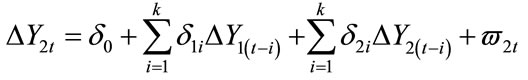
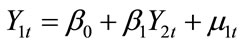
In testing for causality between stock prices, home prices, and private consumption, we draw on the standard [11] causality test, in which the first difference of the dependent variable is regressed on the lagged first differences of both the dependent and the independent variables, as shown below. First differencing of the variables is required in the presence of unit roots in the variables as is shown to be the case for the time series of this paper:
 (1)
(1)
 (2)
(2)
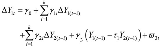
A finding that the coefficients γ2 (d1) are jointly significant indicates unidirectional Granger causality from Y2 to Y1 (from Y1 to Y2). If both coefficients Y2 and d1 are found to be jointly significant, then we have bilateral causality or feedback between Y1 and Y2. However, as shown by [12], the above equation is mis-specified if the underlying variables are cointegrated. Under such conditions, the Granger causality equations should be modified to incorporate the so-called error corrections terms associated with the cointegration equations, as follows:
 (3)
(3)
 (4)
(4)
In the light of the foregoing, it is thus necessary to test the underlying data for the presence of both unit roots and cointegration to determine the appropriate form of the equation to employ in the causality tests. Such tests can be performed using the standard [14] unit root test and the [12] cointegration test.
However, as recent works by [15-17], and [13], among others, show, both the Dickey-Fuller and Engle-Granger tests can yield misleading results in the presence of breaks in the data. In the presence of such breaks, for example, the Dickey-Fuller test may indicate the presence of a unit root in the data, while in reality the data are stationary around a shifting or broken trend. Likewise, such breaks in the data may lead to the Engle-Granger test to incorrectly reject the existence of cointegration between the underling variables. Given that the possibility of breaks in the data is very strong in the present study, as the sample period has been characterized by major events such as oil price shocks and huge drops in stock prices throughout the world, we also employ the recently developed tests which are robust with respect to the presence of breaks in the data.
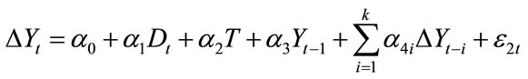
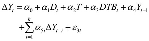
One such test, developed by [17], provides evidence as to whether the data are characterized by unit roots in the context of endogenously determined breaks in the level and direction of the trends in the data. Specifically, we use the following equations to perform tests for unit roots with the respective alternatives being a level shift, and a joint level and slope shift:
 (5)
(5)
 (6)
(6)
where D is a dummy variable with a value of 0 for the periods before the break and 1 thereafter, DTB = T − TB if T > TB and DTB = 0 otherwise, and TB represents the breakpoint. In both equations, the breakpoint is endogenously determined by running recursive regressions and selecting the values of TB for which the coefficient of Y1 is most highly significant, using the critical values provided by [17]. Note that if the dummy variables are dropped from the above equations, i.e., if we exclude the possibility of a break of either kind in the data, the above equations simply reduce to the standard Dickey-Fuller unit root test against the alternative of stationarity around a linear trend.
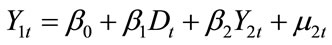
With the time series properties of the data established, we then test for cointegration to determine the appropriate form of the equations of the causality tests. Again recognizing the possibility of breaks in the data, we employ three different cointegrating equations. This first is the basic Engle-Granger test, which is appropriate in a simple bivariate framework, assuming no breaks in the data:
 (7)
(7)
Under this test, cointegration is accepted if the hypothesis of a unit root in the estimated residuals is rejected.
The second model modifies the Engle-Granger equation to test for a level shift in the data:
 (8)
(8)
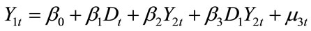
Finally, the third model tests for both a level and a directional shift:
 (9)
(9)
where the dummy variable D is defined as in Equations (5) and (6). Note that here again if the dummy variables are dropped from the above equations, i.e., if we exclude the possibility of a break of either kind in the data, the above equations simply reduce to the standard EngleGranger cointegration test.
Whether the variables of the model are found to be cointegrated or not determines the form of the equation to be employed in the causality tests. If the variables are cointegrated, it is necessary to include the estimated residuals from the above cointegrating equations in the causality tests. Otherwise, a simple VAR in first differences will suffice. Our equations test first whether stock prices cause consumer confidence and then whether consumer confidence causes stock prices. Finding that stock prices drive consumer sentiment, we then perform parallel tests for bilateral causality between consumer sentiment and the economy.
3. Empirical Findings
We perform the tests described above for the US stock prices, home prices, and consumer spending. The underlying data, which are annual and cover the period 1890- 2010, are taken from Shiller [18], are expressed in real terms, and are logarithmic. (The consumption data are also expressed per capita and annualized for the year 2010). Since all the unit root and cointegration tests incorporate lags, we determine the appropriate leg length beginning with lags of 6 years and then use the likelihood ratio test to determine whether a shorter lag is warranted. More specifically, we test downward to see whether each lag is significant and drop the lag if it proves insignificant.
The unit root test results are reported in Table 1. For each country, the Dickey-Fuller test, assuming no breaks in the data, indicate that all variables are I(1). However, considering the possibility that breaks in the data may account for our findings of non-stationarity, we perform additional unit root tests considering first the possibility of a level shift and then the possibility of both level and directional shifts. The test results reveal that even after allowing for possible breaks in the data, the stock and home prices are still characterized by unit roots. However, for consumer spending, a break in the consumption series accounts for the finding of a unit root. Moreover, a close examination of the break indicates that it occurred in the Great Depression year of 1931.
Given the finding that all of our underlying data except consumer spending display unit root characteristics, even after allowing for the possibility of breaks in the data, we test for cointegration before performing causality tests, using the estimation methods described in the preceding section. Of course, the finding that only consumption is trend-stationary indicates that this variable cannot be cointegrated with either of the others, but as a precaution, we nevertheless test for this possibility. This precaution is warranted, given the possibility that the low power of the unit root tests may yield invalid results. The EngleGranger cointegration test results appear in Table 2. Since the test results may have been impacted, depending on which of a pair of variables serves as the dependent variable, we ran regressions with each of the underlying variables as the dependent variable. In no case do we find cointegration using the standard Engle-Granger test. The absence of cointegration, however, could be due to structural changes, so we perform a test for an intercept shift and another for intercept and slope shift. Allowing for such shifts, we nevertheless find no evidence for cointegration. This indicates that our causality tests should be performed as simple VARS in first differences,

Table 1. Dickey-fuller unit root test results.

Table 2. Engle-granger cointegration test results.
without the estimated residuals from the cointegrating equations.
The causality test results appear in Table 3. To ensure a lag length which is both uniform across all causality tests and sufficiently long to capture all the relevant causal effects, we used a lag length of 6 years for all our causality tests. As noted, we test whether stock prices, home prices, and consumer spending are characterized by the presence of bilateral causalities. Our results indicate that there is a bilateral Granger causality between stock and home prices, a bilateral causality between stock prices and consumption, and only a unilateral causality from home prices to consumption.
Having presented our causality test results, we can now offer some interpretation of these findings. As to the effect of stock prices on home values, it is clear that changes in stock prices will affect the household balance sheets, thereby impacting the ability of households to qualify for mortgages and, hence, affecting the household demand for homes. The changes in demand for homes will, in turn, affect their prices. In addition, stock price changes can influence consumer sentiment about the health of the economy [10], which in turn can impact the demand for housing and, hence, home prices. As to the reverse causality from home prices to stock prices, it is common knowledge that changes in home values can change the demand for home equity loans, the proceeds of which can be used to finance the purchases of both assets and goods. To the extent that home equity loans are partially used to acquire more stocks, the prices of stocks will be affected. In addition, changes in demand for goods can impact corporate earnings, again affecting stock prices. In addition, households can directly leverage changes in their home values for margin loans at their brokers, thus providing another channel of influence from home values to stock prices.
As to the bilateral causality between stock prices and consumption, our findings simply provide additional empirical support for the wealth effect of stock prices on consumption, and the effect of consumer spending on
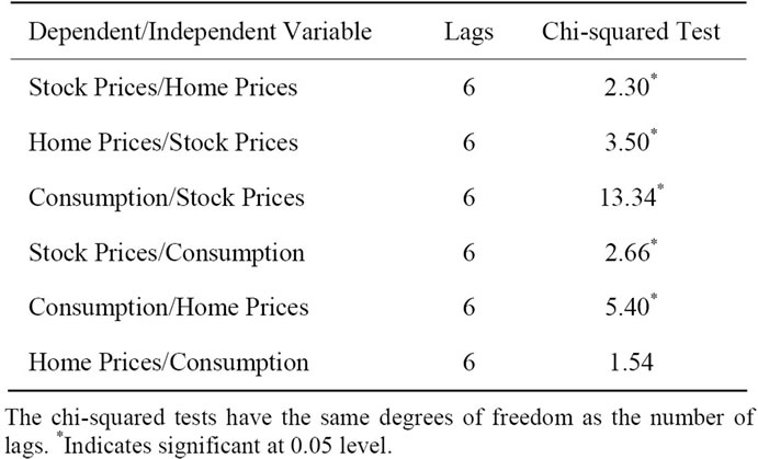
Table 3. Granger causality test results.
corporate earnings and, thus, stock prices.
Finally, concerning the unilateral causality from home prices to private consumption, again we justify our findings based on the wealth effect of home values on consumer spending. Interesting, however, is our finding of a rather weak effect of consumer spending on home prices (with the p-value of 0.16). While it is true that consumer spending can improve general economic conditions and, hence, improve the climate for residential investment, there is little solid theoretical justification that such an effect should be particularly strong. It is our view that investment in housing will depend on longer-term and more permanent changes in such key variables as long term interest rates and “permanent incomes” of the households, which a few years of lags are too short to capture.
4. Conclusions
This paper performs robust bilateral tests of Granger causality between the US stock prices, home prices, and consumer spending. Since the standard Granger causality test, even after incorporating the possibility of non-stationarity and cointegration of the underlying data, can produce misleading results in the presence of structural breaks, we make use of the recently developed unit root and cointegration techniques with breaks to determine the appropriate Granger causal relations between stock prices, home prices, and consumption.
The statistical results indicate bilateral causal relations between stock and home prices and between stock prices and consumption, but only a unilateral causality from home prices to consumption. The results are interesting in that they underline once again the key role of the stock market in driving both home prices and consumer spending in the economy, both because of its direct wealth effect and its indirect effect of serving as a predictor of the future economic conditions. At the same time, our results indicate that the performance of the stock market itself can in turn be impacted through the feedback effects of both the real estate market and the economy in general. In this light, an argument can be made that the improved performance of the US stock market, brought about either through improved corporate performance or appropriate government policies, will constitute an important step in overcoming the recent economic and financial crisis.
REFERENCES
- J. Benjamin, P. Chinloy and D. Jud, “Real Estate Versus Financial Wealth in Consumption,” Journal of Real Estate Finance and Economics, Vol. 29, No. 3, 2004, pp. 341-354. doi:10.1023/B:REAL.0000036677.42950.98
- B. Bosworth, “Phase II: The US Experiment with an Incomes Policy,” The Brookings Papers on Economic Activity, Vol. 2, 1972, pp. 343-383. doi:10.2307/2534181
- K. E. Case, J. M. Quigley and R. J. Shiller, “Stock Market Wealth, Housing Market Wealth, Spending and Consumption,” Working Paper 8606, National Bureau of Economic Research, Cambridge, 2001.
- M. Friedman, “A Theory of the Consumption Function,” Princeton University Press, Princeton, 1957.
- F. S. Mishkin, “Illiquidity, Consumer Durable Expenditure, and Monetary Policy,” American Economic Review, Vol. 66, No. 4, 1976, pp. 642-654.
- P. Temin, “Did Monetary Forces Cause the Great Depression?” Norton, New York, 1976.
- R. E. Hall, “Stochastic Implications of the Life Cycle- Permanent Income Hypothesis: Theory and Evidence,” Journal of Political Economy, Vol. 86, No. 6, 1978, pp. 971-987. doi:10.1086/260724
- C. D. Romer, “The Great Crash and the Inset of the Great Depression,” Quarterly Journal of Economics, Vol. 105, No. 3, 1990, pp. 335-346. doi:10.2307/2937892
- H. Shirvani and B. Wilbratte, “Does Consumption Respond More Strongly to Stock Market Declines than to Increases?” International Economic Journal, Vol. 14, No. 3, 2000, pp. 41-49.
- H. Shirvani and B. Wilbratte, “The Bivariate Causality between Stock Prices and Consumption: International Evidence,” International Quarterly Journal of Finance, 2001.
- C. W. J. Granger, “Investigating Causal Relations by Econometric Models and Cross-Spectral Methods,” Econometrica, Vol. 37, No. 3, 1969, pp. 424-438. doi:10.2307/1912791
- R. F. Engle and C. W. J. Granger, “Co-Integration and Error Correction: Representation, Estimation, and Testing,” Econometrica, Vol. 55, No. 2, 1987, pp. 251-276. doi:10.2307/1913236
- C. W. J. Granger, B.-N. Huang and C.-W. Yang, “A Bivariate Causality between Stock Prices and Exchange Rates: Evidence from, Recent Asian Flu,” Quarterly Review of Economics and Finance, Vol. 40, No. 3, 2000, pp. 337-354. doi:10.1016/S1062-9769(00)00042-9
- D. A. Dickey and W. A. Fuller, “Distribution of the Estimators for Autoregressive Time Series with a Unit Root,” Journal of the American Statistical Association, Vol. 74, No. 366, 1979, pp. 427-431. doi:10.2307/2286348
- P. Perron, “The Great Crash, the Oil-Price Shock, and the Unit-Root Hypothesis,” Econometrica, Vol. 57, No. 6, 1989, pp. 1361-1401. doi:10.2307/1913712
- P. Perron and T. Vogelsang, “Nonstationarity and Level Shifts with an Application to Purchasing Power Parity,” Journal of Business and Economic Statistics, Vol. 10, No. 3, 1992, pp. 301-320. doi:10.2307/1391544
- E. Zivot and D. W. Andrews, “Further Evidence on the Great Crash, the Oil Price shock, and Unit Root Hypothesis,” Journal of Business and Economic Statistics, Vol. 10, No. 3, 1992, pp. 251-270. doi:10.2307/1391541
- R. Shiller, Yale University Homepage, Online Data File, 2011. http://www.econ.yale.edu/~shiller/data.Htm
NOTES
*Corresponding author.