Application of the Hierarchical Functions Expansion Method for the Solution of the Two Dimensional Navier-Stokes Equations for Compressible Fluids in High Velocity

doi:10.4236/epe.2017.92007

Energy and Power Engineering
Vol.09 No.02(2017), Article ID:74207,14 pages
10.4236/epe.2017.92007

Thadeu das Neves Conti¹, Eduardo Lobo Lustosa Cabral², Gaianê Sabundjian¹

●How to Cite this Article

¹Instituto de Pesquisas Energéticas e Nucleares (IPEN), São Paulo, Brazil

²Escola Politécnica da Universidade de São Paulo (USP), São Paulo, Brazil

This work is licensed under the Creative Commons Attribution International License (CC BY 4.0).

http://creativecommons.org/licenses/by/4.0/

Received: December 12, 2016; Accepted: February 14, 2017; Published: February 17, 2017

ABSTRACT

This work presents a new application for the Hierarchical Function Expansion Method for the solution of the Navier-Stokes equations for compressible fluids in two dimensions and in high velocity. This method is based on the finite elements method using the Petrov-Galerkin formulation, know as SUPG (Str- eamline Upwind Petrov-Galerkin), applied with the expansion of the variables into hierarchical functions. To test and validate the numerical method proposed as well as the computational program developed simulations are performed for some cases whose theoretical solutions are known. These cases are the following: continuity test, stability and convergence test, temperature step problem, and several oblique shocks. The objective of the last cases is basically to verify the capture of the shock wave by the method developed. The results obtained in the simulations with the proposed method were good both qualitatively and quantitatively when compared with the theoretical solutions. This allows concluding that the objectives of this work are reached.

Keywords:

Computational Fluid Mechanics, Compressible Flow, Finite Elements Method, Navier-Stokes Equations, Shock Waves

1. Introduction

The solution of complex problems in fluid mechanics and heat transfer with the use of numerical techniques, known as Computational Fluid Dynamics (CFD), is today a reality due to the development of computers with high velocity and with large capacity of data storage. The use of computer codes in some areas of engineering is today a reality and it has been received much attention by numerical researches [1] . The solution of turbulent flow on wings using high capacity computer in 1960 would consume years of processing with a coast of millions of dollars. Today, the solution of this kind of problem using modern computers would consume only few minutes of CPU with a coast of hundred dollars.

This work develops an application of the hierarchical function expansion method, elaborated by [2] , for the solution of Navier-Stokes equations in two dimensions for high velocity compressible flows. This method consists on the use of the finite element method with a Petrov-Galerkin formulation and the expansion of the variables in hierarchical functions. The use of hierarchical expansion allows changing the degree of the adjustment polynomial of the variables during the calculation process without restarting the simulation. Moreover, the numerical method developed has the great advantage of being able to adapt the degree of polynomial until the necessary value, instead of using extremely refined meshes.

In a general way, the classical method of the weighted residuals (Galerkin) is used to get the equations for calculating the coefficients of the expansion functions. However, it is observed that in problems of convective-diffusive transport with convection predominant the Galerkin method fails. Thus, normally for these problems, it is used the Petrov-Galerkin formulation [3] where the weighting functions are different from the expansion functions.

The Petrov-Galerkin formulation consists on the method known as SUPG (Streamline Upwind Petrov-Galerkin) developed by [3] . In this method, the wei- ghting functions are building by adding a perturbation term in the weighting functions used in the Galerkin formulation. This perturbation acts only in the direction of the fluid flow [2] . Note that the SUPG method presents stability and very accurate results. The expansion functions used in the method developed in this work are formed by Legendre Polynomials which are adjusted in the elements in order to define corner, side and area functions. The main reason to use in this work the Legendre Polynomials instead of orthogonal functions such as sine, cosine and exponential, is because only a few functions are necessary to adjust to the shapes of complex solutions. This happens because a polynomial is much more complex than others functions like sine and exponential and comparatively it has a higher capacity of curve fitting. It is observed, however, that smaller is the number of functions used for the expansion of the variables simpler the numerical method becomes.

2. Theoretical Development

As mentioned the numerical method proposed in this work consist on the application of the hierarchical functions expansion method for the solution of pro- blems for compressible fluid flow at high velocities in two dimensions. The method proposed in this work uses the Continuity, Momentum and Energy conservation Equations together with the Mass Velocity and State Equations. These equations are all in two dimensions, x and z directions. These equations are the commonly used and are the following:

Continuity Equation:

(1)

Momentum Equations:

(2)

(3)

Energy Equation:

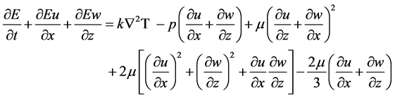(4)

Mass velocity Equations:

(5)

(6)

State Equation:

(7)

Total energy Equation:

(8)

For the flow solution the physical domain is divided into a mesh of several elements. These elements can have an arbitrary shape. However, in this work rectangular elements are used.

For each elements i, j of the solution domain the variables, u, w, G_x, G_z_,, E, p and T are described by a function expansion as follows:

(9)

where M is the total number of expansion functions used for describing each variables, N_m is m^th expansion function for the element i, j and are respectively the coefficients of the variables, u, w, , , E, p e T correspondent to the m^th expansion function for the element ij of the mesh. It is emphasized that depending on the degree of the expansion, or of the number of expansion functions used the solution, the accuracy of the solution can be adjusted.

The solution of the conservation Equations is easier if a local (element) coordinate system is used. This local coordinate system also allows easily modifying the method to use irregular geometries without great modifications. The local space coordinates are denoted by ξ and η. The correspondence of the coordinates ξ and η with the Cartesian coordinates, x and z, for the element i, j of the mesh is given by:

(10)

(11)

It is observed that both ξ and η change from −1 to +1 inside each element. Asmentioned the coordinates ξ and η are local coordinates of each element. The derivatives of ξ and η with respect to the x and z coordinates are given by:

(12)

(13)

The weighting functions (P_m) follow the consistent Petrov-Galerkin formulation given by [3] . Thus for each element i,j of the mesh the weighting functions are given by:

(14)

Equations (1) to (8) are manipulated using several steps. 1) First the variables are substitute by the expansions given by Equation (9). 2) The equations are weighted and integrated inside each element of computational domain. 3) The time derivatives of the variables are approximation by a backward difference. 4) The Green’s Theorem is used to transform the diffusion terms of the momentum and energy equations into first order terms. 5) The equations are written in matricial form for each element i,j of the solution domain. After this process the final equations are given by Equations (15) to (22) presented next.

Continuity Equation:

(15)

Momentum Equation in the x direction:

(16)

Momentum Equation in the z direction:

(17)

Energy Equation:

(18)

Mass velocity Equation in the x direction:

(19)

Mass velocity Equation in the z direction:

(20)

State Equation:

(21)

Total energy Equation:

(22)

The hierarchical expansion functions used in this work are based on the Legendre Polynomials adjusted in the rectangular elements in a very convenient form. The association of the expansion functions to the elements is performed in such a way to define corner, side and area functions. The expansion functions associate with the sides and the area of the elements can have the necessary or the desired degree. In this work the expansion functions are prepared to use degrees from one to six. The Gauss-Quadrature method is used to calculate the integrals involved in Equations (15) to (22). It is emphasized that even so the maximum degree of the expansion functions adopted in this work is limited to six it is possible to increased the expansion degree. This may be necessary for problems that demand fine solution details.

Figure 1 presents a typical rectangular element and the parameters associated with the corners (1, 2, 3, 4), sides (L_x e L_z), and area (A_n) functions.

Note that for Equations (15) to (22) be used to solve a flow problem it is necessary that the Equations for neighbor elements are put together to have only one equation for each variable of the solution domain. In [4] gave the details concerning this agglutination process.

3. Results

For the application of the numerical method proposed a computer code was developed to simulate flow problems. With the objective to apply and analyze the numerical method proposed in this work some known cases of the literature are simulated. These cases are the following: tests of consistency and stability, problem of the temperature step and problem of the oblique shock. The fluid used in these cases is air with the following the viscosity (μ = 2 × 10^-⁵ kg/ms) and the thermal conductivity (k = 2 × 10^-² J/msK) are considered constants.

Figure 1. Two-dimension rectangular element and itsassociated parameters.

Consistency and stability test. The first case simulated consists on the verification of consistency and stability of the numerical method. This verification is performed with the simulation of a normal shock wave in supersonic flow. It is important to emphasize that in this test the shock wave is not dynamically capture. This means that the shock wave reproduced is only a reproduction of the boundary conditions used for the problem.

Figure 2 presents the computational domain for this problem. The boundary conditions for the lower left side, that characterize region 1, represent the flow conditions before the shock. The boundary conditions for the lower right side, that characterize region 2, represent the flow conditions after the shock. The dotted line represents the position of the normal shock that divides the domain in the two regions.

The boundary conditions for region 1 (before the shock) are: temperature, T₁ = 300 k; pressure, p₁ = 1 bar; velocity in the x direction, u₁ = 694 m/s (normal velocity with respect to the shock line); and velocity in the zdirection, w₁ = 0 m/s (tangential velocity with respect to the shock line). The boundary conditions for region 2 (after the shock) are: temperature, T₂ = 506.4 k; pressure, p₂ = 4.2 bar; velocity in x, u₂ = 260.2 m/s (normal velocity with respect to the shock line);and velocity in z, w₂ = 0 m/s (tangential velocity with respect to the shock line). The boundary conditions for the velocities, pressure and temperature for region 2 (after the shock) are obtained by the jump equations given by [5] . Figure 3 presents the results calculated for the normal velocity with respect to the shock. The interface colors represent velocity ranges whose values can be seen in the scale of the graph.

This test was simulated with three different meshes. One mesh contains 100 cells, the other contains 400 cells, and the last mesh contains 1600 cells. The

Figure 2. Computational domain (1.2 m × 1.2 m) of the test of convergence and stability.

Figure 3. Result of the velocity normal to the shock for the normal shock problem. The computational meshused is composed of 1600 cells in the direction z to degree 2 of the expansion of polynomials.

result shown in Figure 3 is obtained with the 1600 cells mesh. Note, as it was expected, that as the number of cells in the mesh increases the numerical solution approaches the correct solution, mainly near the interface between regions 1 and 2.

Temperature step problem. The second case analyzed verifies the problem of numerical diffusion, or false diffusion, that may artificially created by the numerical method. This case consists on the simulation of a temperature discontinuity (step) in a supersonic flow. The temperature step is formed by the boundary conditions imposed by problem. The problem of false diffusion is verified mainly in convection predominant problems. Figure 4 shows the computational domain used for this problem.

The boundary conditions imposed for this problem consists on specifying the flow conditions in the left and lower sides. For the left side, region 1, the boundary conditions are: temperature, T₁ = 310 k; pressure, p₁ = 1 bar; velocity in x, u₁ = 500 m/s; and velocity in z, w₁ = 500 m/s. For the lower side, region 2, the boundary conditions are given by: temperature, T₂ = 290 k; pressure, p₂ = 1bar; velocity in x, u₂ = 500 m/s; and velocity in z, w₂ = 500 m/s. Note that, with the purpose to generate the temperature step, the boundary condition for the temperature differs 20 k between the left and the lower sides.

The fluid properties used in this case are: non-viscous fluid, that is m = 0, and thermal conductivity, k = 0. Zero viscosity and zero thermal conductive eliminate the phenomena of diffusion both in the momentum and in the energy equations. Thus, any diffusion that may appear in the solution is caused by numerical problems. This makes easy to detect the problem of false diffusion.

The boundary condition used for the fluid velocity in the left and lower sides of the solution domain in this case is equal. Thus an interface at 45^˚ between the two temperature regions must appear in the solution. Note that the boundary conditions for the components of the velocity vector in the left and lower sides may be different. Using different velocity components in the left and lower sides changes the angle of the different fluid conditions with respect to the x direction

Figure 4. Computational domain (2.0 m × 2.0 m) for the step temperature problem.

and, therefore, the relative direction between the mesh and the fluid flow. The case analyzed in this section has an angle of 45˚, but [4] presents the results for other case with different angles.

Figure 5 shows the behavior of the temperature in regions 1 and 2 and the interface of the supersonic flow imposed by the boundary conditions. For this test a 100 cells mesh was used with different degrees of expansion. First, second, third and fourth order expansion degrees were used. As expected, the result obtained with the fourth order expansion is the one that better approximates the correct solution. The small fluctuation in the temperature of region 2 is due to difficult and slow convergence of the numerical method.

Oblique shock wave. This problem consists on a supersonic flow that hits on a body surface obliquely, forming an oblique shock wave. The objective of this problem is to dynamic capture a straight line oblique shock wave with non natural solution, or forced solution (intense shock). Other cases of oblique shock waves were simulated with the method developed, such as, the capture of a straight line oblique shock wave with natural solution (weak shock) and, the capture of a curve and dislocated shock wave resulting from the oblique shock of a fluid with and obstacle. In this paper only the intense shock wave is present, the other cases can be seen in [4] .

Figure 6 shows the solution domain used for this problem. The boundary condition for the left side and the first 2/3 of the lower side (region 1) of the solution domain is Mach number, M₁ = 2.9, and the direction of the flow with respect to the body surface forms an angle θ₁ = 11.3˚. The boundary conditions for the right side and the last 1/3 of lower side (region 2) of the solution domain is a pressure, p₂ = 9.6 bar.

Figure 5. Results for the temperature in the temperature step problem. The computa- tional mesh has 100 cellsin the x and z directions andthe variable expansion have fourth order degree.

Note that the natural solution for an oblique shock wave would be obtained by imposing only the flow velocity at the borders of region 1. Due to the imposition of the pressure at the borders of region 2 the forced solution (intense shock solution) is obtained. In the forced solution the angle of inclination of the formed shock wave is greater than that for the case of the natural solution.

The computational mesh used for this case is the same used in previous case, i.e., nine elements in both x and z directions, with x = z = 0.33 m. The steady state solution is obtained running a false transient with a time step, t = 10⁻⁵ s. A second degree expansion is used for the problem variables.

According to [6] (table of oblique shock, appendix D), with M₁ = 2.9, θ₁ = 11.3˚ and pressure p₂ = 9.6 bar, the resulting oblique shock wave has an angle of inclination with respect to the x direction, β, equals to 85˚. These conditions form the forced solution (intense shock solution) for an oblique shock problem. The objective of this test is then to verify if the method developed is capable of capturing the shock wave with the right inclination as given by the theoretical result presented by [6] . Figure 7 shows the results of this test where the red color represents the region before the shock, the blue after the shock and the yellow the interface of the shock.

As expected the results of Figure 7 show an oblique shock wave. The shock wave formed is not a perfect straight line, as expected from the theoretical solution, and its inclination angle is 79, 5˚ with respect to the x direction (the correct theoretical angle is 85˚). The error in the inclination angle is caused by the boundary condition imposed on the superior boundary located at z = 1 m, which has the conditions for the flow before the shock. Note that the curve formed in

Figure 6. Computational domain (1.0 m × 1.0 m) for the oblique shock problemwith for- ced solution.

Figure 7. Result of the flow velocity showing the capture oblique straight line shock wave (forced solution).

the shock wave near the superior boundary is also caused by this problem with the boundary conditions. The mesh used for this problem had 9 cells and the expansion degree was the second order.

As mentioned before, many others cases including consistency and stability tests and oblique and normal shocks were simulated with the method developed and they are presented in [4] .

4. Conclusion

Simulations of supersonic flows, incident obliquely on a body, it was realized to verify the capacity of the numerical method developed in to simulate, adequately, compressible fluid flow in high velocity and to capture shock wave. Through the done analysis, in function of the results obtained in the simulations realized, it can be concluded that the objective of this work was reached in satisfactory way, because the results obtained with the numerical method developed in this work, it was qualitatively and quantitatively goods, when compared with the found theoretical results in literature.

Cite this paper

das Neves Conti, T., Cabral, E.L.L. and Sabundjian, G. (2017) Application of the Hierarchical Functions Expansion Method for the Solution of the Two Dimensional Navier-Stokes Equations for Compressible Fluids in High Velocity. Energy and Power Engineering, 9, 86-99. https://doi.org/10.4236/epe.2017.92007

References

1. Maliska, C.R. (1995) Transferência de Calor e Mecânica dos Fluidos Computacional. LTC-Livros Técnicos e Científicos Editora S.A., Rio de Janeiro.

2. Zienkiewicz, O.C. and Morgan, K. (1983) Finite Elements and Approximation. University of Wales, Swansea, New York.

3. Brooks, A.N. and Hughes, T.J.R. (1982) Streamline Upwind Petrov-Galerkin Formulation for Convection-Dominated Flows with Particular Emphasis on the Incompressible Navier-Stokes Equations. Computer Methods in Applied Mechanics and Engineering, 32, 199-259.
https://doi.org/10.1016/0045-7825(82)90071-8

4. Conti, T.N. (2006) Application of Hierarchical Functions Expansion Method for the Solution of the Two Dimensional Navier-Stokes Equations for Compressible Fluids in High Velocity. Ph.D. Thesis, Mechanical Engineering Department, University of São Paulo, São Paulo.

5. Simões-Moreira, J.R. (2002) Teoria do Escoamento Compressível. Apostila da disciplina Escoamento Compressível, Departamento de Engenharia Mecânica, Escola Politécnica da Universidade de São Paulo.