Advances in Pure Mathematics
Vol.07 No.08(2017), Article ID:78128,24 pages
10.4236/apm.2017.78025
A Note on Kuratowski’s Theorem and Its Related Topics
K. P. Shum
Institute of Mathematics, Yunnan University, Kunming, China

Copyright © 2017 by author and Scientific Research Publishing Inc.
This work is licensed under the Creative Commons Attribution International License (CC BY 4.0).
http://creativecommons.org/licenses/by/4.0/


Received: June 22, 2017; Accepted: July 31, 2017; Published: August 3, 2017
ABSTRACT
In point set topology, it is well known that the Kuratowski 14-set problem is one of the most interesting results. In this note, we first give a brief survey of the Kuratowski’s theorem. In particular, we will study and investigate the structure of the boundary of a given subset in a topological space. Some new results and topics which are related to the theorem of Kuratowski are presented and discussed. Finally, we pose some open problems of Kuratowski- type.
Keywords:
Kuratowski 14-Set, Kuratowski’s Theorem

1. Introduction
The problem of Kuratowski 14-sets was first proposed in 1922 by the famous Polish mathematician Kazimierz Kuratowski who discovered that at most 14 distinct sets can be generated by applying the closure operator and the com- plementation operator on a subset A of a topological space X in any order repeatedly (see [1] ). We now call a subset A in a topological space a K-set if A can generate 14 distinct sets by taking closure and complementation on A in any order. To find an example of a K-set in the real line is posed to many mathematics students all over the world, usually in the class of elementary general topology. The students can easily check that the set is a K- set (see [2] ). Another interesting example of a K-set in the real line is the set [3] [5] .
Now, we denote the complementation of the set A by . As , where e is the identity operator, and so . We des- cribe this fact by saying that the operator c has the involution property, more- over if , then . Also,we use to denote the closure of the set A. It means the smallest closed set containing A. According to Kura- towski, the closure operator has the following properties:
i) , (the closure of a void set).
ii) , (the expansion property).
iii) , (the idempotent property).
iv) , (the additivity property).
In point set topology, we usually use to denote the closure of a set A. However, for the sake of convenience, in dealing with the algebraic closure of a set A, we simply use to denote the closure of the set A. Thus, both and are used to denote the closure of a set A. Now, we also use the notation and to denote the interior of a set A. For the sake of sim- plicity, We write B as the complement of the set A.It is clear that is the complete of . With the applications of the algebraic closure operator, It is well known that the interior of the set A is the set . Since B is used to denote , we now list the family of 14 sets generated by A in Table 1.

Table 1. The family of 14 sets generated by A.
In order to illustrate the inclusion relationship of the above 14 sets, we give the following relationship diagram. As the relationship diagram would look quite bulky if we put all the set inclusion symbols in the diagram. Thus, for the sake of simplicity, we use “®” to mean the inclusion relationship in the diagram. This nice relationship diagram was first given in Kuratowski in [1] (Diagram 1).

Diagram 1. The inclusion relationship of the 14 sets.
The papers [3] - [8] are closely related to the Kuratowski’s theorem. The paper of Gardner and Jackson in [9] gave detailed description and information of the Kuratowski 14 set problem. The papers [3] [10] - [23] also studied and investigated the problems which are closely related to the closure and interior operators of a given set.
2. Algebraic Operator and the Algebraic Interior Operators
Throughout this section, we use and to denote the algebraic closure operator, respectively. According to Kuratowski [3] , the algebraic closure operator has the following properties:
i) Monotonic property, i.e., if , then ,
ii) Expansive property, i.e., ,
iii) Idempotent property, i.e., ,
iv) Additive property, i.e., .
On the other hand, the algebraic interior operator has the following pro- perties:
a) Monotonic property, i.e., if , then ,
b) Shrinking property, i.e., ,
c) Idempotent property, i.e., , i.e., ,
d) Additive property, i.e., .
Consider . By using the above properties of algebraic closure operator and the algebraic interior operator, we obtain immediately the following crucial theorem.
Theorem 2.1. Let be the closure and interior operators. Then we derive the following identities, and .
Proof. By using the shrinking property of , we have . By applying the monotonic property and the idempotent property of , we can easily deduce the equations . On the other hand, because we have , consequently, we derive that . Recall that and , by acting these two identities in the above equations, we obtain . Thus, our theorem is proved. ,
Corollary 2.2. Because and . We immediately see in the above Table 1, we have , . Since the sets , , , , , , , and , , , , , , are possibly distinct. We therefore conclude that at most 14 distinct sets can be generated by taking closure and complementation operator on the set , repeatedly in any order.
Let be subsets of a given set . Then, by applying the complementation operator on these two sets. we have the following properties:
a) The inversion property, If , then , we simply denote this situation by .
b) The involution property, , i.e., , the identity.
c) The separation property. Since , , we simply denote this case by .
Now, we consider the complementation operator c on a bounded lattice , where 0 is the minimum element of the lattice L and 1 is the greatest element of the lattice L. In general, the bounded lattice can be regarded as a power set of a give set L, if , then we write . The can always be regarded as the zero function. We notice that if , then , . Moreover, if and , then we always have .
For the complementation operator c, we have the following theorem.
Theorem 2.3. Let be a complementation operator and the identity operator on a bounded lattice . Then and .
Proof. The proof is quite easy. For the sake of the interest of the readers, we provide here two proofs.
Proof i). Because , c is clearly surjective and injective. Thus, for , by the inversion property of c, i.e., , we have and hence . Now, by the involution property of c, we deduce that .
Proof ii). Suppose that for any . Then we have . This contradicts to , . Hence, there exists such that . Consequently, , . Therefore, . The proof is now completed.
3. The Boundary of a Subset in a Topological Space
For any subset A in a topological space, the boundary of A is defined by . Hence, the boundary operator of A is denoted by . Similarly, we can define the rim operator, and the side operator by . Obviously, the boundary operator, the rim operator and the side operator are closely related on a distributive lattice. It is noted that we always have , . It is obvious that the boundary, the rim and the side of a subset A in a topological space are different concepts. The following example is an example of the above three notations.
Example 3.1. Let be a closed-open interval in the real line . Then according to the definitions of the boundary, the rim and the side of the given set in a topological space , we immediately see that , and . It is clear that the above three concepts are dis- tinct concepts, in fact, the rim and the side of a subset in are parts of the boundary of .
It is noteworthy that the sequence of powers of s is sometimes infinite(for , ).
In the following example, we construct an infinite sequence of side operator.
The construction of such an infinite sequence of side operator in a subset of positive integers is quite technical.
Example 3.2. We first consider the set , . Now, we make a bounded lattice . In this bounded lattice , “0” is the empty set and “1” is the set itself. The operation “ ” can be regarded as the set union and the operation “ ” can be regarded as the set intersection. Consider the subsets in this bounded lattice .
Let be the set of all positive integers. For all , let , denoted by with . Consider the set
Now for . Define . Then, we can
easily verify that is an algebraic closure operator of , where
is the power set of the set . We first take . Then we
have , and ; , and so
, .
Thus, for , we have . This shows that is an infinite sequence.
We now call an expansive operator g a quasi algebraic closure operator if but . Obviously, the quasi algebraic closure operator is a generalized algebraic closure operator. Naturally, one would ask whether the Kuratowski’s theorem still holds for the quasi algebraic closure operator?
In the following example, we show that Kuratowski’s theorem does not hold for the quasi algebraic closure operator.
Example 3.3. For any arbitrary integer , consider the subset
We first let be the power set of the real line .
Define the function by
and
Now, we define a function as follows:
where, . Then, after verification, we can easily see that if , then , also . Thus, g is an expansive operator.
By the definition of the operator g again, we can verify that but . Hence, g is indeed a quasi algebraic closure operator.
Let . Then by applying the operator g on the set , we have .
Applying c and g by repetition on the above equality, we obtain the following sequence of sets:
Thus, it is clear that is an infinite sequence of sets.
This example illustrates that the theorem of Kuratowski does not hold anymore for quasi algebraic closure operators.
For the boundary operator and the rim operator, we have the following theorem. (see [24] )
Theorem 3.4. (i) (ii) .
Proof of i):
Thus we have . . On the other hand, by , we deduce that , and Math_209#. Hence, we have proved that .
Proof of ii): Clearly, . Also by , we have and thereby we obtain . Thus, we deduce that , and consequently .
Remark. The amalgamation of the boundary operator with the other algebraic operators also produces a number of useful equalities. (see [25] )
Proposition 3.5. (i) .
Proof. By , , . Hence we have . Consequently,
This implies that . Thus, .
Remark 3.6. Using the equalities , , , we can easily deduce that , , , (that is, the zero operator), , , , , , , , , , etc.
Finally, we consider some questions which are closely related to the theorem of Kuratowski.
Let be subsets of a space M. Then we call an operator an algebraic quasi-complmentation operator if satisfies the separation property , , simply denoted it by ; also sa- tisfies the inversion property, i.e., if , then , we simply denote this situation by , but does not satisfies the involution property, , i.e., , the identity
We now pose the following question.
Question 3.7. a) Let be a given subset in a topological space . How many distinct sets can be generated by applying the algebraic closure operator and the algebraic quasi-complementation operator successfully on in any order?
b) Likewisely, we call a shrinking operator an algebraic quasi-interior operator if but not .Can we construct an algebraic quasi- interior open set for the set , that ?
Now, we ask when will an algebraic quasi-interior operator and the complementation operator generate a finite semigroup under the usual operator composition?
In order to help answer the above questions, we construct an algebraic quasi-complementation operator .
Let be a real line. For any element , define , and . Obviously, ; and because if ,then , but Thus, is indeed an algebraic quasi- complementation operator.
By using the idea of algebraic quasi closure operator described in Example 2.6, one can therefore construct an algebraic quasi interior operator. Hence, by the idea of the construction of an algebraic quasi interior operator, the reader should be able to answer the above questions.
4. Further Relationship of Algebraic Closure and the Algebraic Interior Operations
We notice that an equivalent formulation of the Kuratowski’s theorem is that at most 7 distinct sets can be obtained by the composition of the algebraic closure operator and the algebraic interior operator . In order to show clearly the mutually inclusion relationship of these 7 distinct sets composed by and on a given set . we give again the following Hasse diagram (Diagram 2).

Diagram 2. The inclusion relationship of 7 distinct sets.
For a given subset A in a topological space X, we call the sets generated from A by successive applications of the algebraic closure and complementation operations in any order on A the relatives of A. Thus, by Kuratowski’s theorem, a K-set A always have 14 relative sets.
It is natural to ask whether there exists a subset in a topological space with less than 14 relative sets? The following theorem gives an answer to the above question.
Theorem 4.1. If the rim of a set is nowhere dense, then by successive applications of closure operator and complementation operator, in any order, on , has at most 10 relative sets.
Proof. We first denote the interior of the set by . Then . Consequently, by using the algebraic closure operator, we have . Now, . Be- cause the rim of the set , say is nowhere dense, we have and so, . Thus, we see immediately that , that is, . Conversely, implies that . Hence, we deduce that
(1)
Now we put and so on. For , we put , for , put . Also, similarly, we put . For , , . By using Kurato- wski’s theorem again, we always have , . By the equation ob- tained above, we see that . Thus A has at most 10 distinct relative sets.
In the literature, P. Halmos [12] first called a set A a regular open set if . Dually, he called a set B regular closed if . If X is a topological space containing a K-set, then we always have , . This means that the space X simultaneously contains a regular closed set and a regular open set.
The following theorem is also an interesting theorem.
Theorem 4.2. If the rim of a set is dense in a regular closed subset of a topological space , then has at most 12 distinct relative sets by taking the algebraic closure operator and the the complementation operators repeatedly in any order on .
Proof. Let be a regular closed set. Then by definition, we have . Since , by the additive property of the algebraic closure, we have . This is because we assume that is dense in . Now, we have . This leads to , and thereby . Trivially, . Hence, we have proved that , that is, . By the result of Kuratowski’s theorem, we always have , . Thus, we can easily see that has at most 12 distinct relative.
It was stated by D. Sherman [22] that 13 distinct operators can be produced by the combination of the algebraic closure operation , the algebraic interior operation and the intersection operation “ ” on a given set . This result is the answer to the well known problem . If the union operation “ ” is also allowed to use, then D.Sherman in [22] has shown that at most 35 different operators can be derived.This problem is called the pro- blem. The solution of the problem and its dual problem are shown in the following Hasse diagrams [23] (Diagram 3).
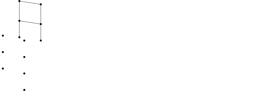
Diagram 3. The solution of the problem and its dual problem
Proof. Let be a regular closed set. Then . Since , by the additive property of the relation “ ” on a given set . This result is the answer to the well known problem . If the union operation “ ” is also allowed to use, then at most 35 different operators can be formed. This problem is now called the problem. The solution of and are shown in the following Hasse diagrams [23] (Diagram 4 and Diagram 5).

Diagram 4.

Diagram 5.
It is clear that the problem is the dual of the problem.
One can verify the following subset of the real line
is a Shermann set, that is, it can generate 13 distinct sets by successively applications of the algebraic closure operator,the algebraic interior operator and the set intersection operations on T in any order (see also [22] ).
5. An Example of Kuratowski 14 Sets in the Set of Positive Integers
Let be the set of all positive integers and . Then Hammer in 1960 defined , where is the set product of copies of . Clearly, and . Thus, is an expansive and ide- mpotent operator, we now call the Hammer closure. Now, we define and call it the Hammer interior operator. It is clear that is also a shrinking and idempotent operator.
The following interesting question was asked by Hammer in 1960 [12] . Do and generated exactly 14 distinct subsets by composition of and in any order, in the set of positive integers? By using the expansive property of and the shrinking property of , we can easily prove that , . Write and . Then we obtain the following 14 distinct sets listed in Table 1.
We now give the following example to answer the open problem of Hammer in 1960. This example was given by Shum in 1996. (see [26] ).
Example 5.1. The following subset of the set of positive integers
is a K-set.
We list bellow the family of all the 14 relatives of the set . This would help the readers to check the validity of the example.
;
;
;
;
;
;
;
;
;
;
;
;
.
The relationship of the above 14 sets can be seen in Diagram 6.
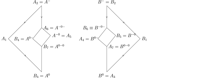
Diagram 6. The relationship of the 14 sets.
Recall that for a subset in the set of positive integers , the Hammer closure of is defined by , where is the set product of n copies of . It is natural to ask how to construct a K-set in the set ? The following lemma gives some ideas and hints.
Lemma 5.2. Let be prime numbers and . If , then , where .
Proof. If , then . This implies that and so we have , a contradiction.
Lemma 5.3. Assume that . Then .
Proof. If , then by our assumption, we have , and so . This leads to , and hence . Consequently, we deduce that , a contradiction.
By using the arguments , , repeatedly, we de- duce the following lemma.
Lemma 5.4. 1) Let be a composite number and is a prime number. If , then ;
2) If or , then ;
3) If , is a composite number, then or , where is a prime number but is not equal to ;
4) If , , then ;
5) is impossible;
6) Let be the prime decomposition length of the composite number . If , then ;
7) is impossible if are both composite numbers.
Proof. The proofs of this lemma are routine but quite tedious, we hence omit the details.
By summing up the above lemmas, we state the following theorem.
Theorem 5.5. If , then is not a K-set.
Proof. The proof is to check case by case. For example, we consider , , , or until all possible cases are exhausted and are impossible. There- fore we conclude that is not a K-set if .
Theorem 5.6. Let be a subset of the set of all positive integers and are prime numbers. Then we have the following statements:
1) If is a K-set, then contains at least five elements and the elements of can be composed of not more than three distinct prime numbers.
2) If is a K-set with five elements, then must be one of the following forms:
a) ;
b) ;
c) ;
d) .
For more information concerning the construction of a K-set, the reader is referred to K. P. Shum [26] .
In view of Diagram 5, there are four distinct sets, namely the sets , , between the sets and . Likewisely, there are also four distinct sets, namely, the sets , , and between the sets and .
Now, we perform the usual set operations of union intersection and subtraction on the above sets, we obtain the following equalities:
1) ;
2) ;
3) ;
4) ;
5)
6) ;
7) .
Because the boundary of a set in the topological space is defined by .
Since the rim of a set is defined by and so . This means that the rim of , is a part of the boundary .
By using the equation and , we immediately see that the gain boundary of . Likewisely, we can also see that the inner boundary of , ; also, the public boundary of , ; the neutral boundary ; the outer boun- dary of , ; the loss boun- dary of
Now, by using the above concepts of the components of the boundary of a set , we obtain the following equalities related to the above components of the boundaries and the 7 Kuratowski sets. (see [26] )
1) ;
2) ;
3) ;
4) ;
5) ;
6) ;
7) .
We now consider the Structure of the boundary of a set in a topological space.
The boundary of a set and all its components in a topological space can be interpreted in the following “envelope diagram” (see [27] ) (Diagram 7).

Diagram 7. The boundary of a set A and all its components in a topological space.
In Diagram 6, can be regarded as a troop of soldiers and is the troop of the enemies of .
In the diagram, is the public boundary at which the troops and are in combatomg.
can be regarded as the ceased fire zone or the negotiation area between the troops and , and therefore, we call this part of boundary the neutral boundary of .
, the inner boundary is the final defence frontier of , that is, it can be regarded as the Mignot defence line of the troop .
, the gain boundary of , it can be interpreted as the picket posts of the troop and these posts will be seized and occupied by the troop when the war begins.
, the outer boundary of which is the inner boundary of the troop . Roughly speaking, the inner boundary of can be regarded as the skin of and the outer boundary can be regarded as the clothes of . Then one can easily distinct the inner boundary and the outer boundary of a set in a given space .
, the loss boundary of which can be described as the gain boundary of the troop .
, the rim boundary of . Of course,the rim of a set is a part of the boundary of the set but it is not necessarily belongs to the given set . In considering the boundary of a set , many people always overlook that there are rims of the set .
Thus,in terms of the closure operator , the interior operator and the complementation operator , we can express the above components of the boundary of the set in the topological space as follows:
We always use the equalities and to describe the different components of the boundary of the set . These different components of the boundary of the set are the followings:
After we have displayed all the possible components of the boundary of a set , we can easily find out the conditions for a set which leads to the set to be a K-set. In fact, we have the following three different types of sets.
Type I. A set is called a standard set if and are all non-empty sets.
One can easily observe that a set is a K-set if and only if is a standard set.
It may happen that .
Type II. A set is called an abnormal set if . It can be observed that an abnormal set is a K-set if and only if and are all non-empty sets.
Type III. A set is called a normal set if . It is clear that a set is a K-set if and only if and are all non-empty, moreover, and may be possibly empty.
Remark 5.7. Because and . In this case, the set is also a standard K-set.
Below are some examples of normal set and abnormal set.
Example 5.8. is a normal set. In this set set, we can check that , , , , , , .
Therefore is a normal K-set.
Example 5.9. The is a abnormal set.
It is clear to see that . Since , , we know that . Because we can easily see that and are all in the interior of . Thus . This shows that is an abnormal set.
The following example is also a standard K-set.
Example 5.10. is a standard set. In this example, , and so . Thus . Be- cause . By using the definitions of the components of the boundary, we can find that , , , , and , . Thus, the boundary of the set has components and so is standard set. We have therefore verified that is indeed a K-set.
6. The K-Sets in a Topological Space
In the above section, we have already considered the construction of a K-set in the set of positive integers. We now turn to the topological space containing a K-set . We concentrate on the so called 7 point space theorem, that is, if is a subset of a n-point space then has at most 2n relations by taking closure and complementation on successively, in any order. This is a significant result in general topology. (see [3] )
Theorem 6.1. Let be a topological space and a K-set in . If exactly 2n distinct sets can be generated by by successive applications, in any order of closure and complementation on , then then the number of the elements of the space can not be less that 7. (see [3] ).
Before we prove this theorem, we recall the process of solving the Kuratowski problem. We first take . Then , and , , and so on.
We first let be the maximum number of distinct sets generated by in the above process of Kuratowski’s theorem.
Similarly, we let be the maximum number of distinct sets generated by in the above process. In order to prove Theorem 5.1, we need the following lemmas.
Lemma 6.2. If , then .
Proof. Let . Then , , and . It is clear to see that is an open set and is contained in . By , we see that is in . Hence, we have . Thus, .
By using the identities and repeatedly, we can prove the following lemmas.
Lemma 6.3. If , then , and .
Lemma 6.4. If , then .
In the above section, we have already discussed the boundary structure of a K-set in a topological space , in particular, we have and . By notice that the neutral boundary of a K-set is non-empty, we can easily verify the following lemma.
Lemma 6.5. If the set is a K-set, that is, the maximal number of relatives is attained, then and .
Now, by using the above lemmas, we can prove Theorem 5.1. In fact, we recall that the standard set, the normal set and the abnormal set can all possibly be the K-set of the required components of the boundary of the set in the topological space all exist, then we see immediately that This result was given by Anusiak and Shum in 1971. (see [3] ). We now state the following theorem for the 7 points space.
Theorem 6.6. Let be an n-point set with . If is a subset of is a K-set under some “good” topology, then the number of non-homomorphic topologies for each can be determined and is shown by the following table (Table 2).
Table 2. The number of non-homomorphic topologies .
In view of the structure of the boundary of a given set and its seven components in a topological space. We can state the following theorem for a K- set in a topological space.
Theorem 6.7. Let be a discrete set in a topological space . If the set is a set, then the cardinality of the set is , conversely, if the cardinality of the set is then it is possible for the set to be a set. However, we still do not know whether will be a set or not if the cardinality of the set is 6 or less.
7. Topics Related to the Closure and Complementation Operators
We now discuss some topics related to the closure and the complementation operators.
(A) Abstract algebras.
By an abstract algebra , we mean a set and a family of fun- damental operations consisting of X-valued functions of several variables run- ning over of and We sometimes write to represent the abstract algebra . If is a non-empty subset of the set , then the smallest subalgebra containing which is closed to an algebraic operator is called the algebraic closure of denoted by of . In application, we call the n-ary operations , where . The smallest class which contains trivial operations and is closed under composition if these fundamental operations is called the class of algebraic operators. The values of constant algebraic operations are called the algebraic constants. We have the following version of Kuratowski’s theorem in the abstract algebra .
Theorem 7.1. can be constructed form by taking the algebraic closure operation and complementation operator successively in any order.
Remark. According to Kuratowski’s theorem,the maximal number of relatives of a subset in an n-element topological space is . However, the same conclusion does not hold in abstract algebra.It should be noted that the classification of topological spaces by using closure and interior operators was also given by C.E. Aull in 1967 (see [4] ).
Example 7.2 Consider the abstract algebra , where , , . Starting with , we have , , . Thus the maximal number generated by is .
By routine verification, we have the following theorem. (see [3] ).
Theorem 7.3. Let be an n-element set. Then there exists an abstract algebra and a subset of such that, by taking algebraic closure and complementation operations to , in any order. We obtain we obtain the following results:
1) relatives of if ;
2) relatives of if ;
3) 14 relatives of if .
The number of relatives of cannot be enlarged.
(B) An application of Kuratowski’s theorem in social science.
Suppose that the immigration rule for the Hong Kong citizens to apply to immigrate to the country is the following:
1) The father can apply himself, his spouses and his dependent children to immigrate with him.
2) The mother can apply herself and her dependent children to immigrate with her.
3) The married son can apply himself, his spouses and his unmarried dependent brothers and sisters in the family to go with him.
4) The married daughter can only apply herself and the unmarried dependent bothers and sisters in the family to go with her.
5) The son in law in the family can only applying himself and his spouses to go with him but not the others.
6) The daughter in law in the family and also the independent children in the family do not have the privilege of application.
Now, Suppose a family have father , mother , son , daughter in law , daughter , son in law , unmarried dependents .
If the following family members first apply to immigrate to UK, then the rest of the family apply next.
The question is how many possible cases will be there for this family in total?
The answer is 14 possible cases because this is a typical application of Kuratowski’s theorem and the algebraic closure operator is the immigration rule .
Let . Then under the above immigration rule, there will be the following 7 cases:
On the other hand, after the father has first applied to immigrate to country . We have the following situations:
and then
Thus, in this immigration application for the family , there are at most 14 distinct combinations (see [18] ).
(C) The Closure and interior operators in general algebras.
Let be the closure operator and , the interior operator acting on a subset in a topological space .
In the literature, a set in a topological space is called a regular open set by Halmos if . Dually, a set in is called regular closed if . Because it has been known in Kuratowski problem that . Thus, if is a K-space, then contains simultaneously a regular closed set and a regular open set. It was also noticed by Shum [28] that the Boolean algebra formed by the set of regular open sets is isomorphic to the Boolean algebra formed by the set of regular closed sets.
We call a mapping an interior operator on the lattice if is a shrinking mapping, i.e., and is an idempotent mapping, i.e., . The mapping is also called meet preserving if .
For the closure operator of a lattice, the reader is referred to [29] .
We give below the following definitions.
Definition 7.4. An interior operator is said to be a strong interior ope- rator if is shrinking, idempotent and meet preserving.
Definition 7.5. A sub semilattice of a complete lattice is called a closed join subsemilattice, if for all and exists then . In general, a closed join sub-semilattice is not necessarily closed. This fact can be seen in the following example (Diagram 8).
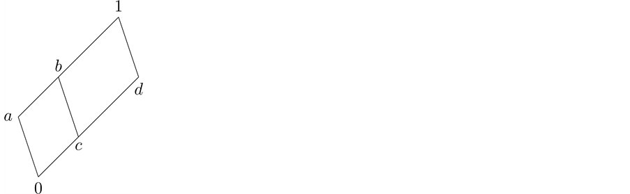
Diagram 8. A closed join sub-semilattice.
In the above lattice, is a join semilattice of . It is clear that . Thus is not a closed join semilattice.
By considering the closed join subsemilattice of a lattice , we obtain the following result related with the Tarski fixed plank. (see [30] [31] and [32] ).
For the strong interior operator on a closed join subsemilattice , we have the following theorem.
Theorem 7.6. The mapping defined by is a strong interior operator on and moreover, , the fixed plank of .
Proof. We first let . Because is a closed join semilattice in . Then from is clearly a strong interior operator on and is also surjective.
Trivially, is a shrinking mapping and for all . Suppose that in . Then we have and . It can be easily verified that leads to . Thus is an expansive mapping. On the other hand we can check that for all , we have and thereby , that is . By the shrinking property of , we have immediately. Thus is a fixed point under the mapping . This means that .
Because , where
. Hence, if we take , then by definition, we have and . Using the expansive property of , we get . Consequently, , that is, . Thus, we have proved that . Again by the shrinking property of , we get . This proves that and hence is an idem- potent mapping.
It remains to prove that the mapping is a meet preserving mapping. Since and , by the shrinking property of again, we have , also by and , we have . Now, we use again the properties of , we deduce that . This proves that is a strong interior operator of . Because . Therefore, we
have shown that , the fixed plank of .
Remark 7.7. Theorem 6.5 can also be extended to topological lattices and further modification of the strong interior operator to the so called topological interior operator. In modifying the strong interior operator to the topological interior operator,the additional requirement is crucial. Thus, the Tarski-like results of subalgebras can also be established in a complete Boolean algebra by using a topological interior operator. It was stated in [34] that if is a subalgebra of a complete Boolean algebra , then we can prove that is a subalgebra of with girth 2,that is, , , where the elements if and only if there exists a topological interior operator and satisfies the equality . We omit the details,The reader is referred to K.P.Shum and A. Yang in [31] and [33] .
(D) Galois connection
Let be the power set of a set , be the power set of a set . If is a relation between the sets and , then, we define the operator and the operator as follows:
Then, we can easily see that
where are the subsets of , are subsets of .
One can prove immediately that if and are partially ordered sets, then the mappings and are the pair of closure operators of and respectively. We now call the pair a Galois connection of the partially ordered sets and . In fact, formed by all the transformations of a three dimensional space then we should be able to use all the invariant classes of to define some kind of geometry and the new geometry will be generated by using some kind of Galois connection pairs. Hence, the affine geometry is closely linked with the invariant classes of geometry under the affine transformations. The relationship of the transformation groups and the invariant classes of geometry under transformations can be regarded as a pair of Galois connection. Thus, we can always make use of group theory to describe the geometry and conversely,we can also describe the extension of fields by using the structures of permutation groups. The set of identities can be used to describe the varieties of algebras concerning invariant properties and vice versa. To link the operation pair (f,i) with some other kinds of Galois connection pairs would be a useful tool in the future to study the recent developing topics in fuzzy algebraic structures, may be in the soft algebraic structures and in theoretical computer Science. There is an increasing need to use some kind of Galois connections to cope with many uncertainty problems of the real world to the existing mathematical systems. The readers are referred to the article on Galois connection by Denecke and Wismath in [34] .
8. Closure in Topological Semigroups
After the concept of Closure introduced by Kuratokski, a topological space was established by using the Kuratowski closure.
Recall that a topological semigroup is a Hausdorff space endowed with a jointly continuous multiplication which is associative on the space. Therefore, the structure of the topological semigroup is closely related to the topological closure of the topological semigroup .
Now, let any . Form the semigroup generated by , that is, . Denote this semigroup by . Take the topological closure closure on . Then is clearly a compact semigroup of . Consider
the set of accumulation points of , that is, . It was
proved by A. D. Wallace in 1955 that is a minimal ideal of and is
also a group. This is the well known theorem of A.D. Wallace [28] in topological semigroup. Another interesting theorem in topological semigroup is the prime ideal theorem of K. Numakura [20] , it states that if is an idempotent element of , then the maximal ideal contained in the open set , namely is an open prime ideal of .
We mention below a theorem concerning the expression of a prime ideal in a compact semigroup.
Theorem 8.1. Let be an open prime ideal in a compact semi- group with . Consider the group , the maximum group generated by the idempotent . Then we have for any group element . In other words, the idempotent element in the open prime ideal can be replaced by any group element .
Proof. We first prove that . If , then there exists . Because is the maximal ideal contained in the open set and hence, the open neighborhood of , namely . Since as well so that the open neighborhood . Now, we let , then we can find an element in the group so that as , a contradiction. Thus we have proved that . Because by definition is the maximal ideal contained in the open set , consequently, we have . This means that we can always replace the idempotent by any group element . Thus, the open prime ideal in the topological semigroup will have more different expressions. The theorem is proved.
For more information concerning the structure of topological semigroups and the properties of ideals and radicals in a topological semigroup, the reader is refereed to the monograph of Wallace [35] and the paper by Shum and Hoo [36] .
In closing this paper, we conclude that the closure and complementation theorem is a very interesting theorem to study, especially the concept of the closure operation has penetrated into many branches in mathematics. My contribution to the Kuratowski Theorem is that I discovered the cardinality of a K-set is seven, that is, a K-set in a topological space contains at least seven points. (see [3] ). I also observe the boundary of a set is composed by Neutral boundary, Public boundary,Gain boundary, Loss boundary,Inner boundary and Outer boundary. This part of work can be seen in Diagram 7 in this paper and in [27] . The example 5.1 given by me is also an interesting finding in the literature.
We now pose the following open questions for solution.
Open problem Let be a subset of the set of integers . Define the Hammer closure of to be , where is a positive integer and is the cartesian set product of copies, under usual multiplication. Let be the set complementation of in .
1) Find a subset in so that will generate exactly 12 distinct sets by taking and successively on in in any order.
2) Find a subset in so that will generate exactly 10 distinct sets by acting and successively on in any order.
We do not have an answer in hand at this moment for this problem, but Theorem 3.3, Theorem 3.4 and also the description of the boundary of the set in a topological space have already given some hints to tackle this problem.
As an exercise, the readers are also encouraged to construct a subset in the real line which will generate exactly 12 distinct subsets and 10 distinct subsets by taking the topological closure operation and the complementation operation, repeatedly on the set in any order.
Cite this paper
Shum, K.P. (2017) A Note on Kuratowski’s Theorem and Its Related Topics. Advances in Pure Mathematics, 7, 383-406. https://doi.org/10.4236/apm.2017.78025
References
- 1. Kuratowski, K. (1922) Sur l’Opération ā de l’Analysis Situs. Fundamenta Mathemathticae, 3, 182-199.
- 2. Steen, L.A. and Seebach, A.J. (1970) Counter Examples in Topology. Holt, Rinehart and Winston, Austin.
- 3. Anusiak, J. and Shum, K.P. (1971) Remarks on Topological Spaces. Colloquium Mathematics, 23, 217-223.
- 4. Aull, C.E. (1967) Classification of Topological Spaces, Bull de l’Acad. Sci Math., Astun. Phys., 15, 773-778.
- 5. Block, N.J. (1977) The Free Closure Algebra on Finite Generators. Indagationes Mathematicae, 80, 362-379.https://doi.org/10.1016/1385-7258(77)90050-6
- 6. Brandsma, H. (2003) The Fourteen Subsets Problem, Interior Closure and Complements in Topology Explained, Topology Attas.http://at.yorku.ca/p/a/c/a/24.htm
- 7. Chapman, T.A. (1962) An Extension of the Kuratowski Closure and Complementation Problem. Mathematics Magazine, 35, 31-35.https://doi.org/10.2307/2689098
- 8. Chapman, T.A. (1962) A Further Note in Closure and Interior Operators. American Mathematical Monthly, 69, 524-529.https://doi.org/10.2307/2311193
- 9. Gardner, B.J. and Jackson, M. (2008) The Kuratowski Closure and Complement Theorem. New Zealand Journal of Mathematics, 38, 9-44.
- 10. Garee, E. and Oliver, J.P. (1995) On Closure Unifying that Interior of a Closed Element Is Closed. Communications in Algebra, 23, 3715-3728. https://doi.org/10.1080/00927879508825428
- 11. Graham, R.L., Knuth, D.E. and Metzin, T.S. (1972) Complements and Transitive Closures. Discrete Mathematics, 21, 17-29. https://doi.org/10.1016/0012-365X(72)90057-X
- 12. Hammer, P.C. (1960) Kuratowski’s Closure Theorem. New Arched Work, 8, 74-80.
- 13. Jackson, M. (2004) Closure Semilattice. Algebra Universalis, 52, 1-37. https://doi.org/10.1007/s00012-004-1871-3
- 14. Knaster, B. (1927) Une Theorem sur es Functions d’Ensembles. Annals of Mathematics, 6, 133-134.
- 15. Kam, S.M. and Shum, K.P. (1992) On a Problem of P.C. Hammer. Southeast Asian Bulletin of Mathematics, 16, 123-127.
- 16. Koenen, W. (1971) The Kuratowski Closure Problem in Topology of Convexity. American Mathematical Monthly, 78, 362-367.
- 17. Langeford, E. (1966) Characterization of Kuratowski 14 Sets. The American Mathematical Monthly, 73, 704-708.
- 18. Moser, L.E. (1977) Closure, Interior and Union on Finite Topological Spaces. Colloquium Mathematicum, 38, 41-51.
- 19. Moslefian, M.S. and Tavalliaii, T. (1995) A Generalization of the Closure-Complement Problem. Punjab University Journal of Mathematics, 58, 1-9.
- 20. Morgando, J. (1960) Some Results on Closure Operators of Partially Ordered Sets. Portugaliae Mathematica, 19, 101-139.
- 21. Peleg, D. (1984) A Generalized Closure and Complement Phenomenon. Discrete Mathematics, 50, 285-293.https://doi.org/10.1016/0012-365X(84)90055-4
- 22. Pigozzi, D. (1972) On Some Operations on Classes of Algebras. Algebra Universalis, 2, 346-353.https://doi.org/10.1007/BF02945045
- 23. Sherman, D. (2010) Varieties on Kuratowski 14 Sets Theorem. American Mathematical Monthly, 117, 113-123.https://doi.org/10.4169/000298910x476031
- 24. Shum, K.P. (1992) The Amalgamation of Closure and Boundary Functions on Semigroup and Algebras of Computer Languages. World Scientific Publishing, Singapore City.
- 25. Numerkura, K. (1957) Prime Ideals and Idempotents in Compact Semigroups. Duke Mathematical Journal, 24, 671-679. https://doi.org/10.1215/S0012-7094-57-02475-4
- 26. Shum, K.P. (1996) Closure Functions on the Set of Positive Integers. Science in China, 39, 337-346.
- 27. Yip, K.W. and Shum, K.P. (1975) On the Structure of Kuratowski Sets. Journal of the Chinese University of Hong Kong, 3, 429-439.
- 28. Tasic, B. (2001) On the Partially Ordered Monoid Generated by the Operators H.S.P.P. on Classes of Algebra. Journal of Algebra, 245, 1-19. https://doi.org/10.1006/jabr.2001.8914
- 29. Ward, M. (1942) The Closure Operators of a Lattice. Annals of Mathematics, 43, 191-196. https://doi.org/10.2307/1968865
- 30. Shum, K.P. (1991) A Characterization for Prime Ideals in Compact Semigroup. Southeast Asian Bulletin of Mathematics, 15, 61-64.
- 31. Shum, K.P. and Yang, A.Z. (1992) Interior Operators and Compact Lattices. Progressive Urban Management Associates, Denver, 73-80.
- 32. Stone, M. (1937) Algebraic Characterizations of Special Boolean Rings. Foundations of Mathematics, 29, 261-267.
- 33. Shum, K.P. and Yang, A.Z. (1998) Complete Subsets and Their Corresponding Functions on a Complete Lattice. Journal of Mathematical Research, 18, 81-86.
- 34. Denecke, K. and Wismath, S. (2014) Galois Conections and Complete Sublattices. In: Denecke, K., Erné, M. and Wismath, S.L., Eds., Galois Connections and Applications, Springer Verlag, Berlin, 211-229.
- 35. Wallace, A.D. (1955) On the Structure of Topological Semigroups. Bulletin of the American Mathematical Society, 61, 95-117. https://doi.org/10.1090/S0002-9904-1955-09895-1
- 36. Hoo, C.S. and Shum, K.P. (1972) On Algebraic Radicals in Mobs. Colloquium Mathematica, 25, 25-35.