Advances in Pure Mathematics
Vol.3 No.9B(2013), Article ID:41122,17 pages DOI:10.4236/apm.2013.39A2002
From Eigenvalues to Singular Values: A Review
Hydrological Service, Jerusalem, Israel
Email: dax20@water.gov.il
Copyright © 2013 Achiya Dax. This is an open access article distributed under the Creative Commons Attribution License, which permits unrestricted use, distribution, and reproduction in any medium, provided the original work is properly cited.
Received August 15, 2013; revised September 15, 2013; accepted September 21, 2013
Keywords: Eigenvalues; Singular Values; Rayleigh Quotient; Orthogonal Quotient Matrices; The Orthogonal Quotients Equality; Eckart-Young Theorem; Ky Fan’s Extremum Principles
ABSTRACT
The analogy between eigenvalues and singular values has many faces. The current review brings together several examples of this analogy. One example regards the similarity between Symmetric Rayleigh Quotients and Rectangular Rayleigh Quotients. Many useful properties of eigenvalues stem are from the Courant-Fischer minimax theorem, from Weyl’s theorem, and their corollaries. Another aspect regards “rectangular” versions of these theorems. Comparing the properties of Rayleigh Quotient matrices with those of Orthogonal Quotient matrices illuminates the subject in a new light. The Orthogonal Quotients Equality is a recent result that converts Eckart-Young’s minimum norm problem into an equivalent maximum norm problem. This exposes a surprising link between the Eckart-Young theorem and Ky Fan’s maximum principle. We see that the two theorems reflect two sides of the same coin: there exists a more general maximum principle from which both theorems are easily derived. Ky Fan has used his extremum principle (on traces of matrices) to derive analog results on determinants of positive definite Rayleigh Quotients matrices. The new extremum principle extends these results to Rectangular Quotients matrices. Bringing all these topics under one roof provides new insight into the fascinating relations between eigenvalues and singular values.
1. Introduction
Let  be a real symmetric
  matrix and let
 be a given nonzero vector. Then the well-known Rayleigh Quotient is defined as
 (1.1)
(1.1)
One motivation behind this definition lies in the following observation. Let  be a given real number. Then there exists an eigenvalue
  of
of  such that
 (1.2)
(1.2)
and the value of  that solves the minimum norm problem
 (1.3)
(1.3)
is given by . In other words,
  provides an estimate for an eigenvalue corresponding to
 . Combining this estimate with the inverse iteration yields the celebrated Rayleigh Quotient Iteration. Other related features are the Courant-Fischer minimax inequalities, Weyl monotonicity theorem, and many other results that stem from these observations. In particular, the largest and the smallest eigenvalues of
  satisfy
 (1.4)
(1.4)
and
 (1.5)
(1.5)
respectively. For detailed discussion of the Rayleigh Quotient and its properties see, for example, [1-41].
The question that initiates our study is how to extend the definition of Rayleigh Quotient in order to estimate a singular value of a general rectangular matrix, where the term “rectangular” means that the matrix is not necessarily symmetric or square. More precisely, let  be a real
  matrix,
  , and let
  and
and  be a pair of nonzero vectors. Then we seek a scalar function of
 , and
, and ,
,  say, whose value approximates the “corresponding” singular value of
 . The answer is given by the Rectangular Quotient,
 (1.6)
(1.6)
where  denotes the Euclidean vector norm. The justifications behind this definition are given in Section 3. It is demonstrated there that the properties of the Rectangular Quotient (1.6) resemble (extend) those of the Rayleigh Quotient (1.1). Indeed, as our review is aimed to show, the above similarity reflects a more general rule: the optimality properties of Orthogonal Quotient matrices resemble (extend) those of Rayleigh Quotient matrices.
Let  be a real
  matrix with
 orthonormal columns. Let
  be a real
 matrix with
  orthonormal columns. Then an
  matrix of the form
 (1.7)
(1.7)
is called an Orthogonal Quotient matrix. Note that
 (1.8)
(1.8)
so the entries of  have the same absolute value as the corresponding rectangular quotients. Matrices of the form (1.7) can be viewed as “rectangular” Rayleigh Quotient matrices. The traditional definition of symmetric Rayleigh Quotient matrices refers to symmetric matrices of the form
 (1.9)
(1.9)
where  and
and  are defined as above, e.g., [20,30,36]. Symmetric Rayleigh Quotient matrices of this form are sometimes called sections. A larger class of Rayleigh Quotients matrices is considered in [34]. These matrices have the form
 (1.10)
where  is a general (nonnormal) square matrix of order
 . The
. The  matrix
  is assumed to be of full column rank, and the
  matrix
  denotes a left inverse of
 . That is, a matrix satisfying
 . Matrices of the forms (1.9) and (1.10) play important roles in the Rayleigh-Ritz procedure and in Krylov subspace methods, e.g., [30,34]. In this context there is rich literature on residual bounds for eigenvalues and eigenspaces. See, for example, [19-21,30,32,34,36]. Another applications of Rayleigh Quotient matrices arise in optimization algorithms that try to keep their approximations on a specific Stiefel manifold, e.g., [6,7,9,35].
A third class of Rayleigh Quotient matrices is obtained from (1.7) by taking . These matrices are involved in residual bounds for singular values and singular spaces, e.g., [2,21].
However, our review turns into different directions. It is aimed to explore the optimality properties of Orthogonal Quotients matrices. Comparing these properties with those of symmetric Rayleigh Quotients matrices reveals highly interesting observations. At the heart of these observations stands a surprising relationship between Eckart-Young’s minimum norm theorem [5] and Ky Fan’s maximum principle [10].
The Eckart-Young theorem considers the problem of approximating one matrix by another matrix of a lower rank. The solution of this problem is also attributed to Schmidt [31]. See [17, pp.~137,138] and [33, p.~76]. The need for low-rank approximations of a matrix is a fundamental problem that arises in many applications, e.g., [3-5,8,14,15,18,33]. The maximum principle of Ky Fan considers the problem of maximizing the trace of a symmetric Rayleigh Quotient matrix. It is also a wellknown result that has many applications, e.g., [1,10-12, 16,22,28]. Yet, so far, the two theorems have always been considered as independent and unrelated results which are based on different arguments. The Orthogonal Quotients Equality is a recent result that converts EckartYoung’s minimum norm problem into an equivalent maximum norm problem. This exposes a surprising similarity between the Eckart-Young theorem and Ky Fan’s maximum principle. We see that the two theorems reflect two sides of the same coin: there exists a more general maximum rule from which both theorems are easily derived.
The plan of our review is as follows. It starts by introducing some necessary notations and facts. Then it turns to expose the basic properties of the Rectangular Quotient (1.6), showing that it solves a number of least norm problems that resemble (1.3). An error bound, similar to (1.2), enables us to bound the distance between  and the closest singular value of
 .
.
Another aspect of the analogy between eigenvalues and singular values is studied in Section 4, in which we consider “rectangular” versions of the Courant-Fischer minimax theorem and Weyl theorem. This paves the way for “traditional” proof of Eckart-Young theorem. Then, using Ky Fan’s dominance theorem, it is easy to conclude Mirsky’s theorem.
The relation between symmetric Rayleigh Quotient matrices and Orthogonal Quotients matrices is studied in Section 5. It is shown there that the least squares properties of Orthogonal Quotient matrices resemble those of symmetric Rayleigh-Quotient matrices. One consequence of these properties is the Orthogonal Quotients Equality, which is derived in Section 6. As noted above, this equality turns the Eckart-Young least squares problem into an equivalent maximum problem, which attempts to maximize the Frobenius norm of an Orthogonal Quotients matrix of the form (1.7).
The symmetric version of the Orthogonal Quotients Equality considers the problem of maximizing (or minimizing) traces of symmetric Rayleigh Quotients matrices. The solution of these problems is given by the celebrated Ky Fan’s Extremum Principles. The similarity between the maximum form of Eckart-Young theorem and Ky Fan’s maximum principle suggests that both observations are special cases of a more general extremum principle. The derivation of this principle is carried out in Section 8. It is shown there that both results are easily concluded from the extended maximum principle.
The review ends by discussing some consequences of the extended principle. One consequence is a minimum-maximum equality that relates Mirsky’s minimum norm problem with the extended maximum problem. A second type of consequence is about traces of Orthogonal Quotients matrices. The results of Ky Fan on traces of symmetric Rayleigh Quotients matrices [10] were extended in his latter papers [11,12] to products of eigenvalues and determinants. The new extremum principle enables the extension of these properties to Orthogonal Quotients matrices.
The current review brings together several old and new results. The “old” results come with appropriate references. In contrast, the “new” results come without references, as most of them are taken from a recent research paper [3] by this author. Yet the current paper derives a number of contributions which are not included in [3]. One contribution regards the extension of Theorem 11 behind the Frobenius norm. Another contribution is the minimum-maximum equality, which is introduced in Section 9. The main difference between [3] and this essay lies in their concept. The first one is a research paper that is aimed at establishing the extended extremum principle. The review exposes some fascinating features of the analogy between eigenvalues and singular values. For this purpose we present several apparently unrelated results. Putting all these topics under one roof gives a better insight into these relations. The description of the results concentrates on real valued matrices and vectors. This simplifies the presentation and helps to focus on the main ideas. The treatment of the complexvalued case should be quite obvious.
2. Notations and Basic Facts
In this section we introduce notations and facts which are needed for coming discussions. As before  denotes a real
  matrix with
 . Let
. Let
 (2.1)
(2.1)
be an SVD of , where
  is an
is an 
orthogonal matrix,  is an
is an  orthogonal matrix, and
  is an
is an  diagonal matrix. The singular values of
  are assumed to be nonnegative and sorted to satisfy
 (2.2)
(2.2)
The columns of  and
and  are called left singular vectors and right singular vectors, respectively. These vectors are related by the equalities
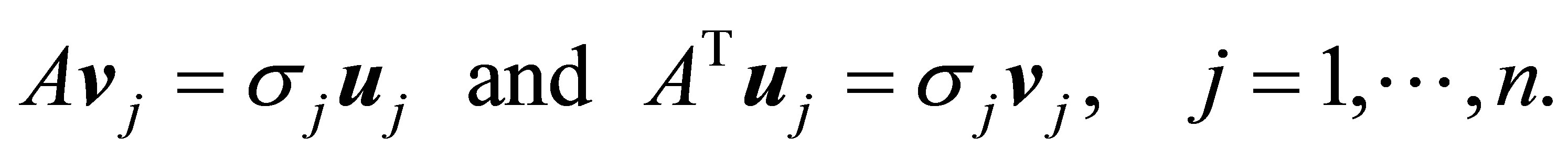 (2.3)
(2.3)
A further consequence of (2.1) is the equality
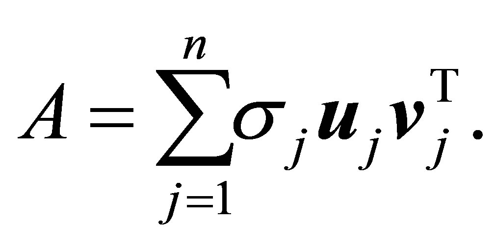 (2.4)
(2.4)
Moreover, let  denote the rank of
 . Then, clearly,
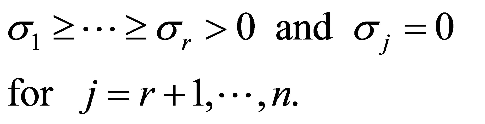 (2.5)
(2.5)
So (2.4) can be rewritten as
 (2.6)
(2.6)
Let the matrices
 (2.7)
(2.7)
be constructed from the first  columns of U and
 respectively. Let
  be a
be a  diagonal matrix. Then the matrix
 (2.8)
(2.8)
is called rank- Truncated SVD of
 .
.
Let , denote the
  entries of the matrices
 , respectively. Then (2.4) indicates that
 (2.9)
(2.9)
and
 (2.10)
where the last inequality follows from the CauchySchwarz inequality and the fact that the columns of  and
and  have unit length.
Another useful property regards the concepts of majorization and unitarily invariant norms. Recall that a matrix norm  on
on  is called unitarily invariant if the equalities
 (2.11)
are satisfied for any matrix , and any pair of unitary matrices
  and
and . Let
. Let  and
and  be a given pair of
  matrices with singular values
respectively. Let  and
and 
denote the corresponding  -vectors of singular values. Then the weak majorization relation
  means that these vectors satisfy the inequalities
 (2.12)
In this case we say that  is weakly majorized by
 , or that the singular values of B are weakly majorized by those of
 . The Dominance Theorem of Ky Fan [11] relates these two concepts. It says that if the singular values of
  are majorized by those of
  then the inequality
 (2.13)
holds for any unitarily invariant norm. For detailed proof of this fact see, for example, [1,11,17,22]. The most popular example of a unitarily invariant norm is, perhaps, the Frobenius matrix norm
 (2.14)
which satisfies
 (2.15)
Other examples are the Schatten  -norms,
 (2.16)
and Ky Fan  -norms,
 (2.17)
The trace norm,
 (2.18)
is obtained for  and
and , while the spectral norm (the 2-norm)
 (2.19)
corresponds to  and
and .
.
Finally, let  and
and  be a pair of positive integers such that
Then
 (2.20)
and
 (2.21)
denote the corresponding Stiefel manifolds. That is,  denotes the set of all real
  matrices with orthonormal columns, while
  is the set of all real
  matrices with orthonormal columns.
3. Rectangular Quotients
Let  be a real
  matrix with
 , and let
 and
and  be a pair of nonzero vectors. To simplify the coming discussion we make the assumptions that
 , and that
  and
and  are unit vectors. That is,
With these assumptions at hand the Rectangular Quotient (1.6) is reduced to the bilinear form
 (3.1)
(3.1)
In this section we briefly derive the basic minimum norm properties that characterize this kind of bilinear forms. We shall start by noting that  solves the one parameter minimization problem
 (3.2)
(3.2)
This observation is a direct consequence of the equalities
and
 (3.3)
(3.3)
Similar arguments show that  solves the least squares problems
 (3.4)
(3.4)
and
 (3.5)
(3.5)
Furthermore, substituting the optimal value of  into (3.3) yields the Rectangular Quotient Equality
 (3.6)
(3.6)
which means that solving the rank-one approximation problem
 (3.7)
(3.7)
is equivalent to solving the maximization problem
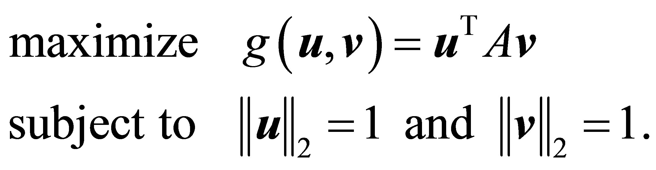 (3.8)
(3.8)
Using the SVD of  the unit vectors in the last problem can be expressed in the form

Therefore, since
 (3.9)
(3.9)
the objective function of (3.8) satisfies
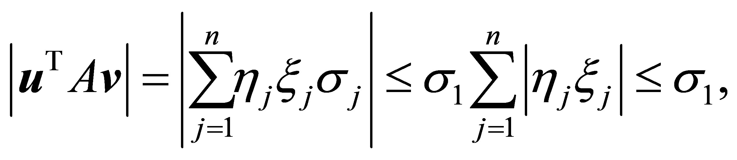
where the last inequality comes from the CauchySchwarz inequality. Moreover, since , this pair of vectors solves (3.8), while
  satisfies
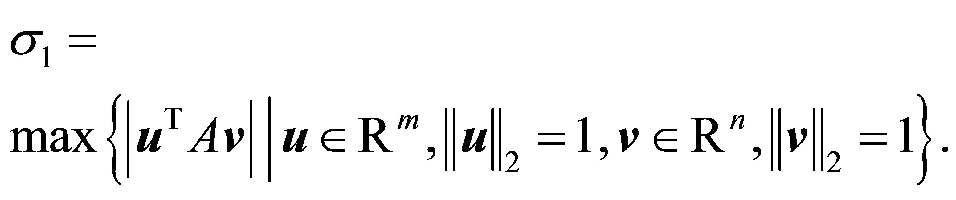 (3.10)
The last result is analogous to (1.4). Yet, in contrast to (1.5), here the orthogonality relations (3.9) imply that
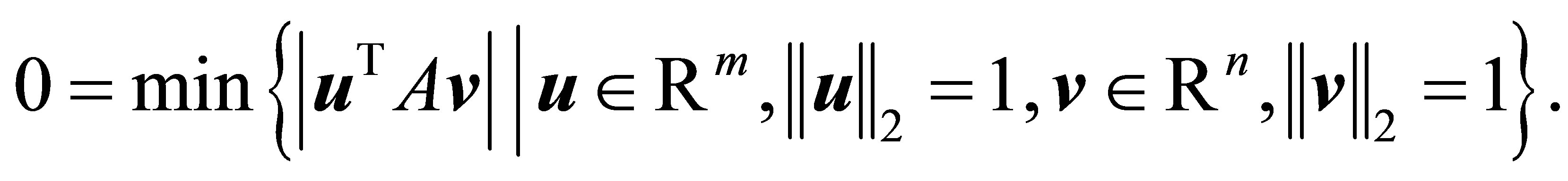 (3.11)
Further min-max properties of scalar rectangular quotients are obtained from the Courant-Fischer theorem, see the next section.
Another justification behind the proposed definition of the Rectangular Quotient comes from the observation that the Rayleigh quotient corresponding to the matrix
 and the vector
  is
is .
.
Hence in this case the bound (1.2) implies the existence of a singular value of ,
,  , that satisfies
 (3.12)
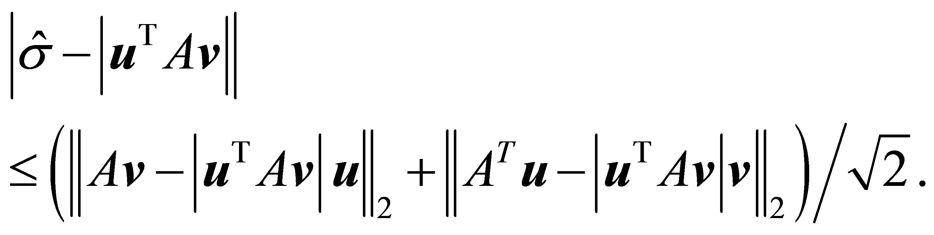
The last bound can be refined by applying the following retrieval rules, derived in [3]. Let  be a given unit vector that satisfies
 , and let
and
provide the corresponding estimates of a left singular vector, and a singular value, respectively. Then
and (3.12) is reduced to
 (3.13)
Similarly let  be a given unit vector that satisfies
 , and let
and
denote the corresponding estimates of a singular vector, and a singular value, respectively. Then here
and (3.12) is reduced to
 (3.14)
We shall finish this section by noting the difference between the Rectangular Quotient (1.6) and the Generalized Rayleigh Quotient (GRQ) proposed by Ostrowski [26]. Let  be a general (nonnormal) square matrix of order n and let
  and
and  be two
  -vectors that satisfy
  where
where  denotes the conjugate transpose of
 . Then the GRQ,
 (3.15)
is aimed to approximate an eigenvalue of  that is “common” to
  and
and . For detailed discussions of the GRQ and its properties see [25-27,29,40].
4. From Eigenvalues to Singular Values
The connection between the singular values of  and the eigenvalues of the matrices ATA, AAT, and
 is quite straightforward. Indeed, many properties of singular values are inherited from this connection. Yet, as our review shows, the depth of the relations is far beyond this basic connection. The Courant-Fischer minimax theorem and Weyl’s theorem provide highly useful results on eigenvalues of symmetric matrices. See [1,30] for detailed discussions of these theorems and their consequences. Below we consider the adaption of these results when moving from eigenvalues to singular values. The adapted theorems are used to provide a “traditional” proof of the Eckart-Young theorem.
As before  denotes a real
  matrix whose SVD is given by (2.1)-(2.7). The first pair of theorems provides useful “minimax” characterizations of singular values. In these theorems
  denotes an arbitrary subspace of
  that has dimension
 . Similarly,
  denotes an arbitrary subspace of
  that has dimension
 .
.
Theorem 1 (Right Courant-Fischer Minimax Theorem)The jth singular value of  satisfies
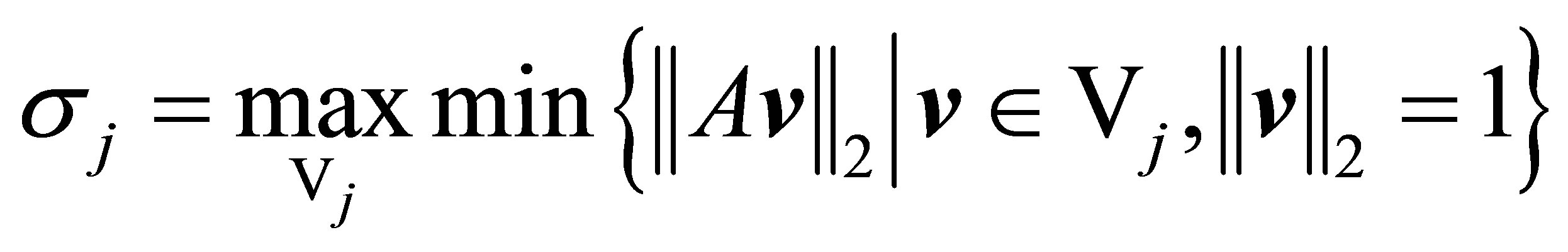 (4.1)
(4.1)
and
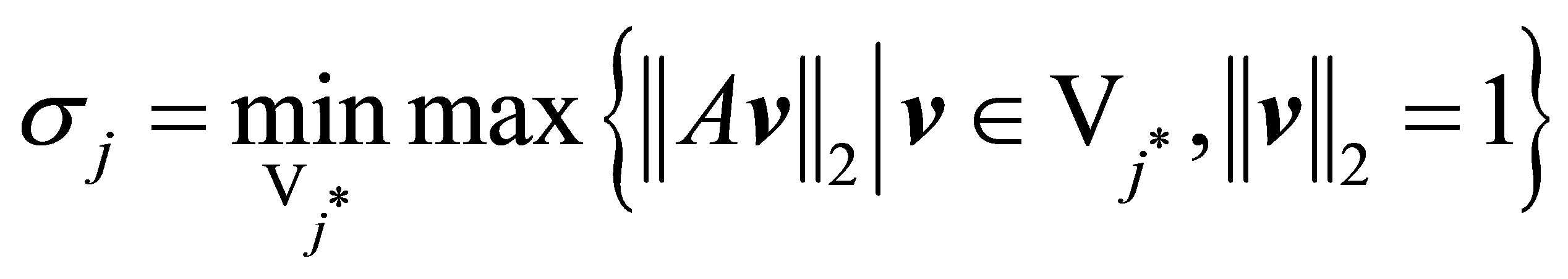 (4.2)
(4.2)
where the integer  is defined by the equality
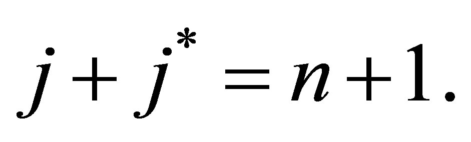 (4.3)
(4.3)
(The maximum in (4.1) is over all  dimensional subspaces
  of
of . The minimum in (4.2) is over all
  dimensional subspaces
  of
of .) Moreover, the maximum in (4.1) is attained for
 , while the minimum in (4.2) is attained for
 .
.
Yet the solutions of both problems are not necessarily unique. 
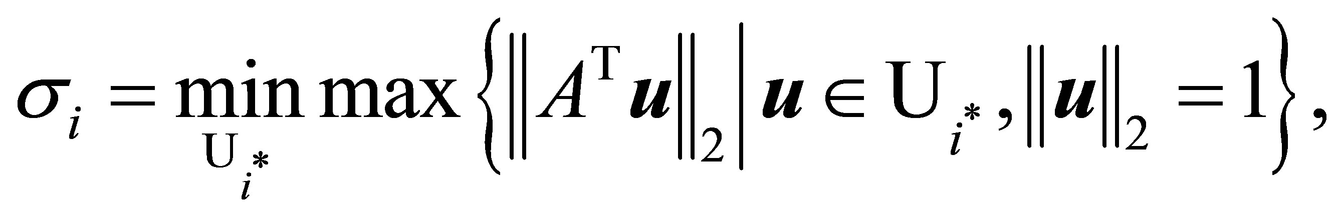
Theorem 2 (Left Courant-Fischer Minimax Theorem) The ith singular value of  satisfies
 (4.4)
(4.4)
and
 (4.5)
(4.5)
where the integer  is defined by the equality
 (4.6)
(4.6)
Moreover, the maximum in (4.4) is attained for
 while the minimum in (4.5) is attained for
 .
. 
Note that Theorem 2 is essentially Theorem 1 for . The proof of Theorem 1 is based on the following idea. The condition (4.3) ensures the existence of a unit vector,
  , that belongs both to
  and
and . Thus
and
So the proof is concluded by verifying that equality holds when using the specified subspaces.
Let  denote another
  real matrix and let
 (4.7)
(4.7)
denote the corresponding difference matrix. The singular values of  and
and  are denoted as
 (4.8)
(4.8)
respectively. The coming corollaries of Theorem 1 answer the question of how the rank of  affects the singular values of
 .
.
Lemma 3 Assume that . In this case
 (4.9)
(4.9)
Proof. Take . Then
  and
and . Consequently
where the last inequality follows from (4.2). 
Theorem 4 (Weyl) Let  and
and  be as in (4.7) - (4.8). Then
 (4.10)
under the convention that  when
when .
.
Proof. Let  be a rank
  Truncated SVD of
 , and let
  to be a rank
  Truncated SVD of
 . Then the largest singular value of
  is
is , while the largest singular value of
  is
is . That is,
 (4.11)
and
 (4.12)
Let the  matrix
  be defined by the equality
Then , and
, and
Hence from (4.11) and (4.12) we see that
where the last inequality follows from Lemma 3. 
Corollary 5 (Majorization) Assume further that , which means
  for
for . Then substituting
  in (4.10) gives
 (4.13)
In other words, if  then the singular values of
  majorize the singular values of
 .
. 
Recall that  denotes a rank-
 Truncated SVD of
 , as defined in (2.8). Roughly speaking the last corollary says that a rank-
 perturbation of
  may cause the singular values to “fall” not more than
  “levels”. The next corollary shows that they are unable to “rise” more than
  levels.
Corollary 6 Observe that (4.7) can be rewritten as  while
while  has the same singular values as
 . Hence a further consequence of Theorem 4 is
 (4.14)
Moreover, if  then
then
 (4.15)

The next results provide useful bounds on the perturbed singular values.
Corollary 7 (Bounding and Interlacing) Using (4.10) and (4.14) with  gives
gives
 (4.16)
and
 (4.17)
Furthermore, consider the special case when  is a rank-one matrix. Then using (4.13) and (4.15) with
  gives
gives
 (4.18)
where  and
and .
. 
Theorem 8 (Eckart-Young) Let  and
and  be as in (4.7)-(4.8) and assume that
 . Then
 (4.19)
Moreover, let  be a rank-
 Truncated SVD of
 , as defined in (2.8). Then
  solves the minimum norm problem
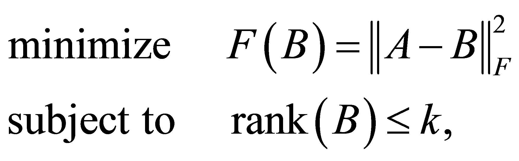 (4.20)
giving the optimal value of
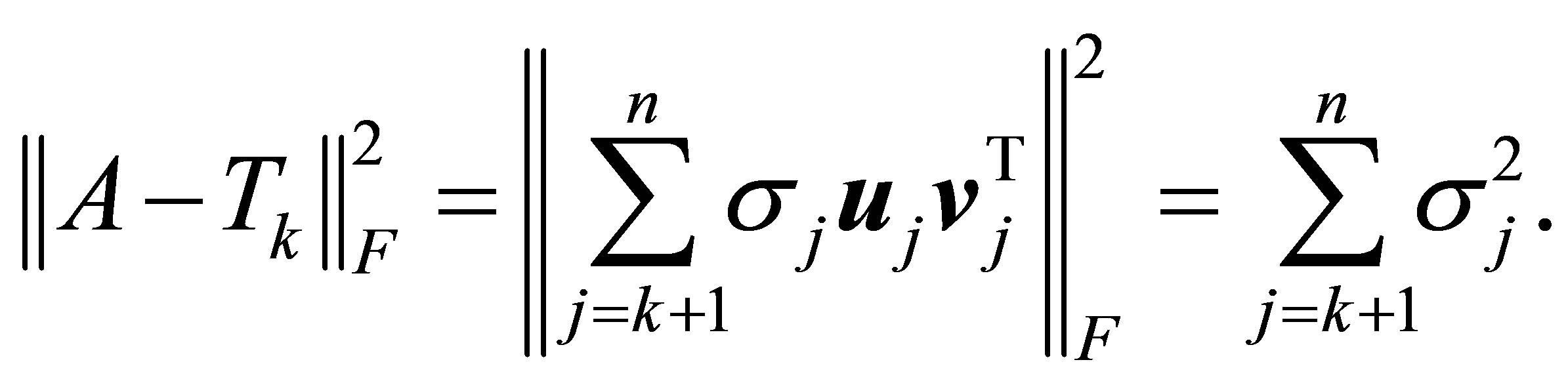
Proof. Using (4.13) we see that
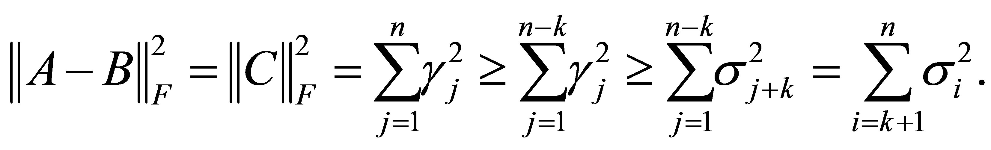

The last theorem says that  is a best rank-
 approximation of
 , regarding the Frobenius norm. Observe that Lemma 3 proves a similar claim for the 2- norm. The next extension is due to Mirsky [23].
Theorem 9 (Mirsky) Let  denote a unitarily invariant norm on
 . Then the inequality
 (4.21)
holds for any matrix  such that
 . In other words,
  solves the minimum norm problem
 (4.22)
Proof. From Corollary 5 we see that the singular values of  majorize those of
 . Hence (4.21) is a direct consequence of Ky Fan Dominance Theorem.
Another related problem is
 (4.23)
where  denotes the set of all real
  matrices of rank
 . Below we will show that the residual matrix
 (4.24)
solves this problem. In other words,  is the smallest perturbation that turns
  into a rank-
 matrix.
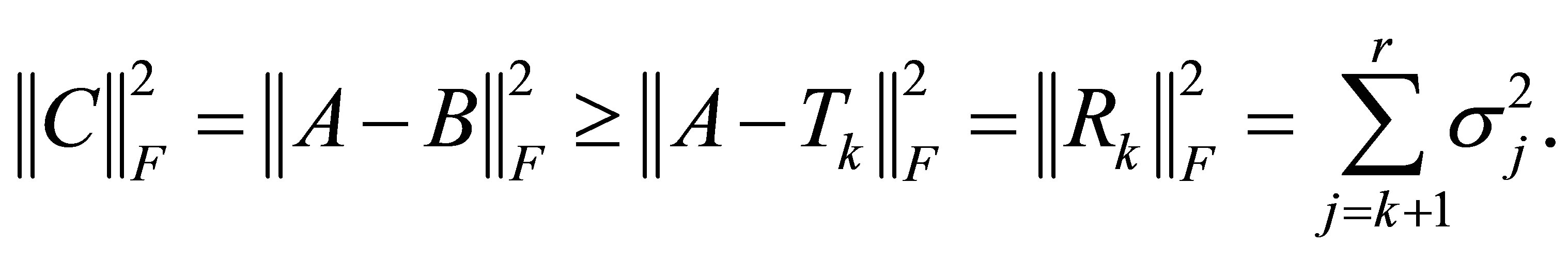
Theorem 10 Let  and C be as in (4.7) and assume that
Then
 (4.25)
Proof. Using the Eckart-Young theorem we obtain

Observe that  remains the solution of (4.23) when this problem is defined by any other unitarily invariant norm. Note also that Total Least Squares problems give rise to a special form of (4.23) in which
 . In this case the solution matrix,
  , is reduced to the rank-one matrix
 , e.g., [14,15]. Further consequences of the Eckart-Young theorem are presented in Section 6.
5. Least Squares Properties of Orthogonal Quotients Matrices
The optimality properties of symmetric Rayleigh Quotient matrices form the basis of the celebrated RayleighRitz procedure, e.g., [30,34]. In this section we derive the corresponding properties of Orthogonal Quotients matrices. As we shall see, Orthogonal Quotient matrices extend symmetric Rayleigh Quotient matrices in the same way that Rectangular Quotients extend Rayleigh Quotients.
Theorem 11 Let
 and
and 
be a given pair of matrices with orthonormal columns, and let
 (5.1)
(5.1)
denote the corresponding orthogonal quotient matrix. Then  solves the following three problems.
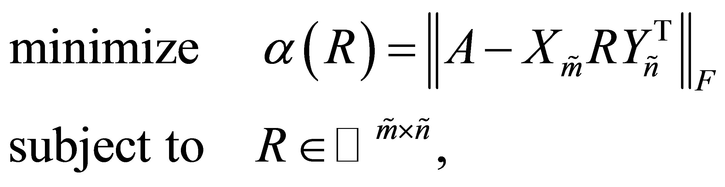 (5.2)
(5.2)
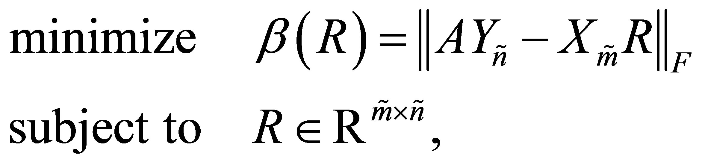 (5.3)
(5.3)
and
 (5.4)
(5.4)
Proof. Completing the columns of  to be an orthonormal basis of
  gives an orthogonal
  matrix,
  , whose first
  columns are the columns of
 . Similarly there exists an orthogonal
  matrix,
  , whose first
  columns are the columns of
 . Therefore, since the Frobenius norm is unitarily invariant,
 (5.5)
(5.5)
where
 (5.6)
(5.6)
The validity of the last equality is easily verified by noting that the  matrix
  is composed of the first
  columns of the
  identity matrix, while the
  matrix
  is composed of the first
  rows of the
  identity matrix. Note also that the corresponding principle submatrix of
  is
is . Hence the choice
  minimizes
 .
.
The other two problems are solved by similar arguments, using the equalities
 (5.7)
(5.7)
and
 (5.8)
(5.8)
where
 (5.9)
(5.9)

Remark A further inspection of relations (5.7)-(5.9) indicates that  solves problems (5.3) and (5.4) even if the Frobenius norm is replaced by any other unitarily invariant matrix norm. However the last claim is not valid for problem (5.2), since “punching” a matrix may increase its norm. To see this point consider the matrices
 and
and , whose trace norms are 2 and
 , respectively. That is, punching
  increases its trace norm. Nevertheless, punching a matrix always reduces its Frobenius norm. Hence the proof of Theorem 11 leads to the following powerful results.
Corollary 12 Let  denote the set of all real
  matrices that have a certain pattern of zeros. (For example, the set of all tridiagonal matrices.) Let the matrix
  be obtained from
  by setting zeros in the corresponding places. Then Theorem 11 remains valid when
  and
and  are replaced by
  and
and  , respectively.
Corollary 13 Assume that  and let
denote the set of all real diagonal  matrices. Let
  and
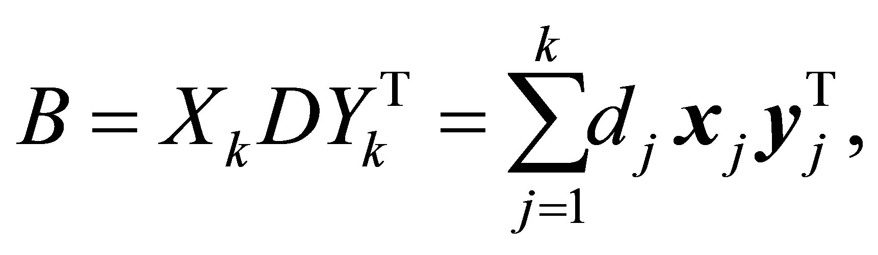
and  be a given pair of matrices with orthonormal columns. Then the matrix
 (5.10)
solves the following three problems.
 (5.11)
 (5.12)
and
 (5.13)

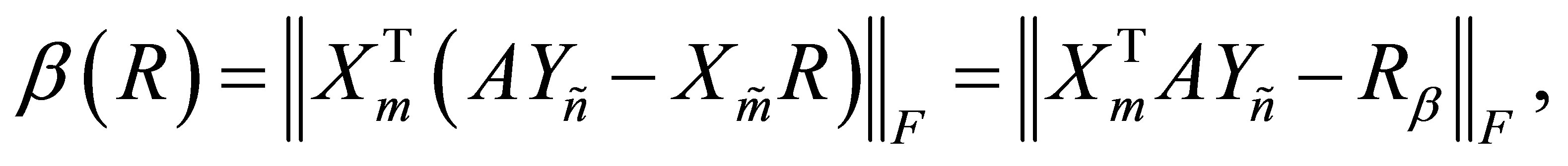
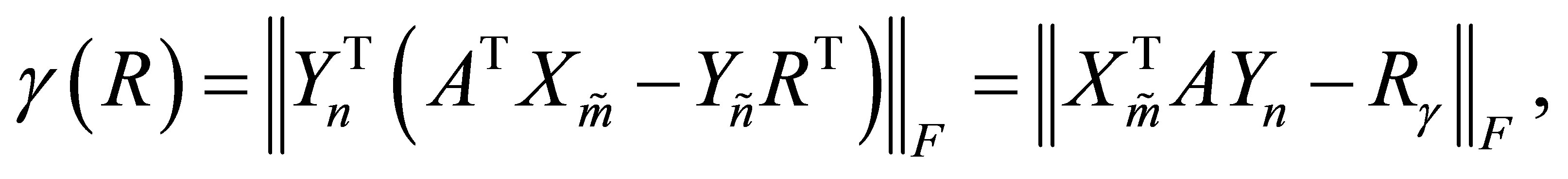
As in the scalar case, the residual functions,  and
and , enable us to bound the “distance” between the singular values of
  and
and . Assume for a moment that
  and let
  denote the singular values of
 . Then there exists a permutation
  of
of  such that
 (5.14)
see [2,21]. The relations (5.7)-(5.9) indicate that the minimal values of  and
and  equal the Frobenius norm of the corresponding off-diagonal blocks in the matrix
 . The next observations regard the minimal value of
 .
.
6. The Orthogonal Quotients Equality and Eckart-Young Theorem
In this section we derive the Orthogonal Quotients Equality and discuss its relation to the Eckart-Young theorem.
Theorem 14 (The Orthogonal Quotients Equality) Let  and
and  be a given pair of matrices with orthonormal columns. Then
 (6.1)
(6.1)
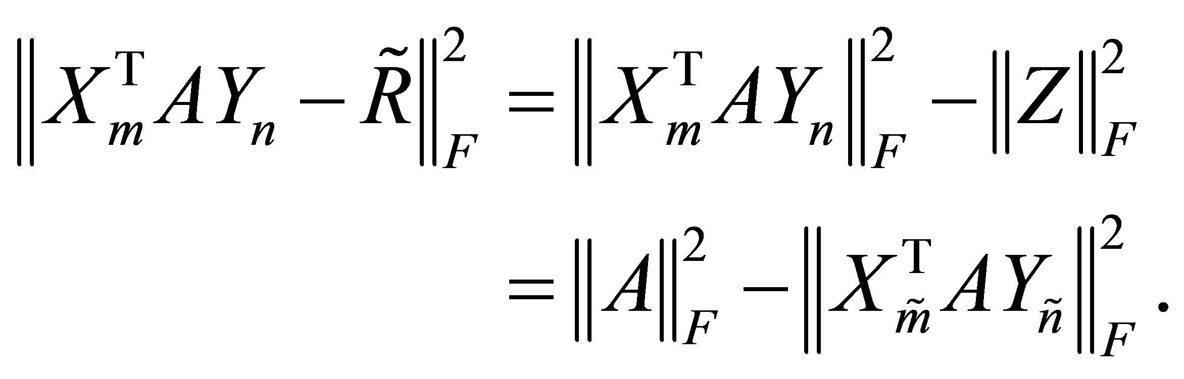
Proof. Following the proof of Theorem 11 we see that
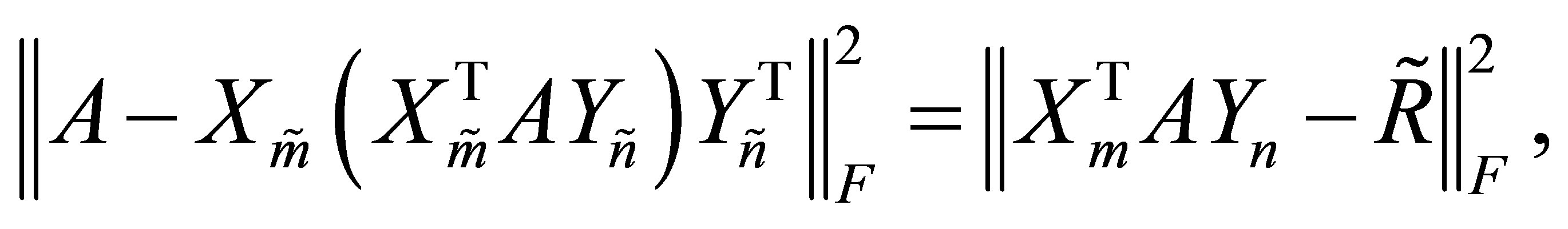 (6.2)
(6.2)
where
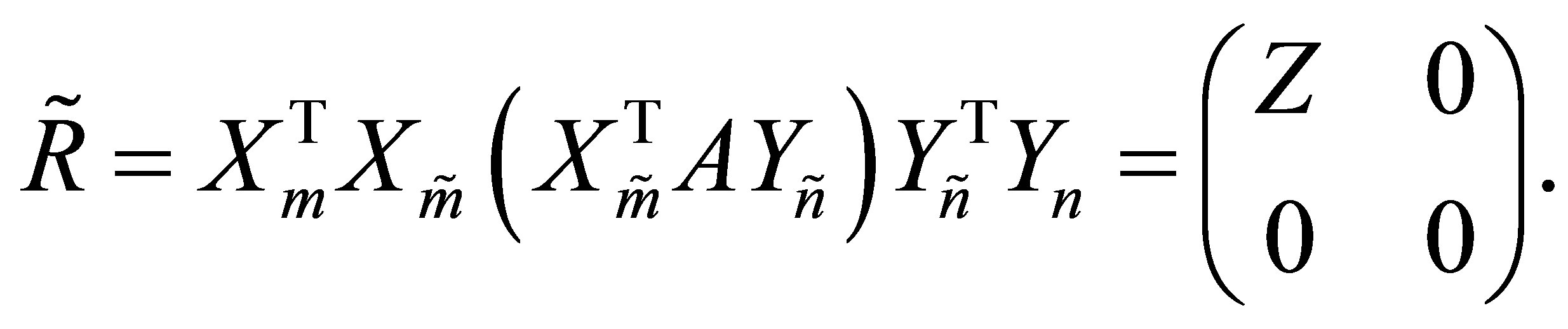
Therefore, since  is a principal submatrix of
 ,
,
Corollary 15 Let  be any
  matrix whose entries satisfy the following rule: Either
 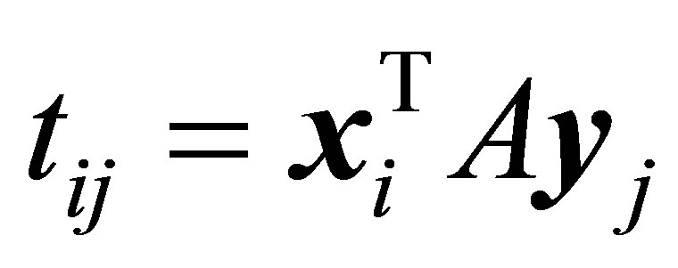 or
or
 . In other words,
  is obtained from
  by setting some entries to zero. Then
 (6.3)
(6.3)
Corollary 16 (The Orthogonal Quotients Equality in Diagonal Form) Let  and
and  be a given pair of matrices with orthonormal columns. Then the diagonal matrix (5.10) satisfies
 (6.4)
(6.4)
In vector notations the last equality takes the form
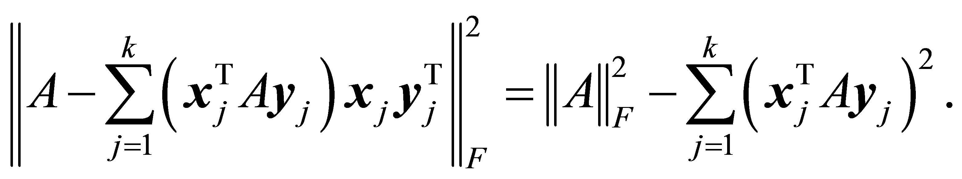 (6.5)
(6.5)

Let us return now to consider the Eckart-Young problem (4.20). One way to express an  matrix, whose rank is at most
 , is
, is
 (6.6)
(6.6)
where ,
,  and
and . Alternatively we can write
  in the form
 (6.7)
(6.7)
where  is a real diagonal
  matrix. (The first form results from complete orthogonal decomposition of
 , while the second form is obtained from the SVD.) Substituting (6.6) in the objective function of (4.20) results in the function
 . Hence, by Theorem 11, there is no loss of generality in replacing
  with
with . Similarly D can be replaced with
 , the solution of (5.11). These observations lead to the following conclusions.
Theorem 17 (Equivalent Formulations of the EckartYoung Problem) There is no loss of generality in writing the Eckart-Young problem (4.20) in the forms
 (6.8)
(6.8)
or
 (6.9)
(6.9)
Moreover, both problems are solved by the SVD matrices  and
and . (See (2.1)-(2.7) for the definition of these matrices.)
The objective functions of the last problems form the left sides of the Orthogonal Quotients Equalities
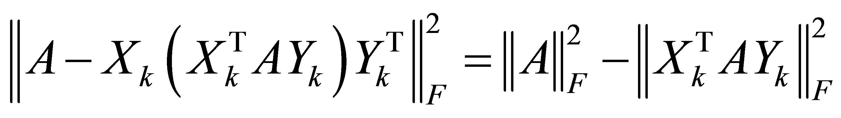 (6.10)
and
 (6.11)
These relations turn the minimum norm problems (6.8)-(6.9) into equivalent maximum norm problems.
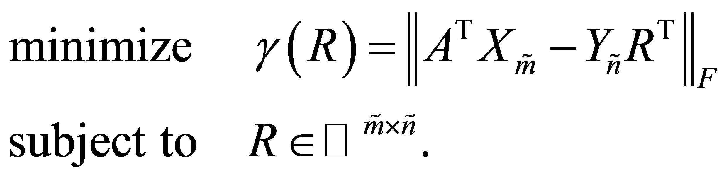
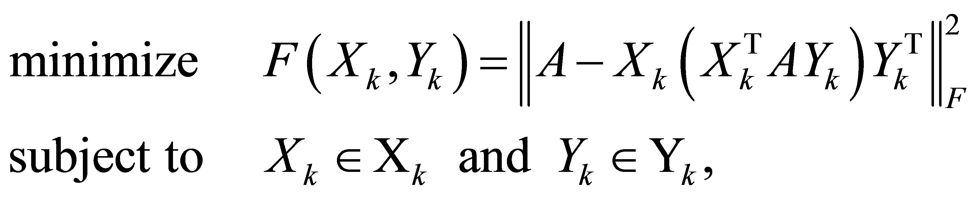
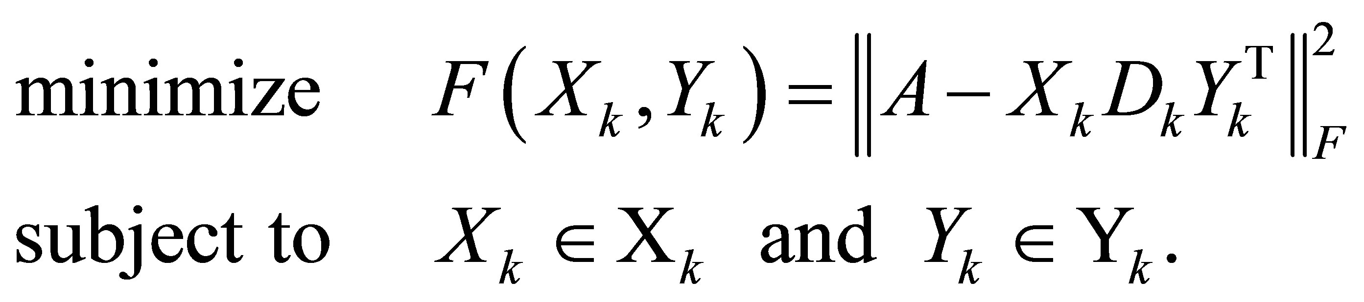
Theorem 18 (Maximum Norm Formulations of the Eckart-Young Problem) The Eckart-Young problems (6.8) and (6.9) are equivalent to the problems
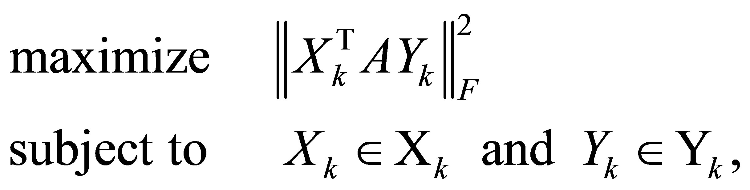 (6.12)
and
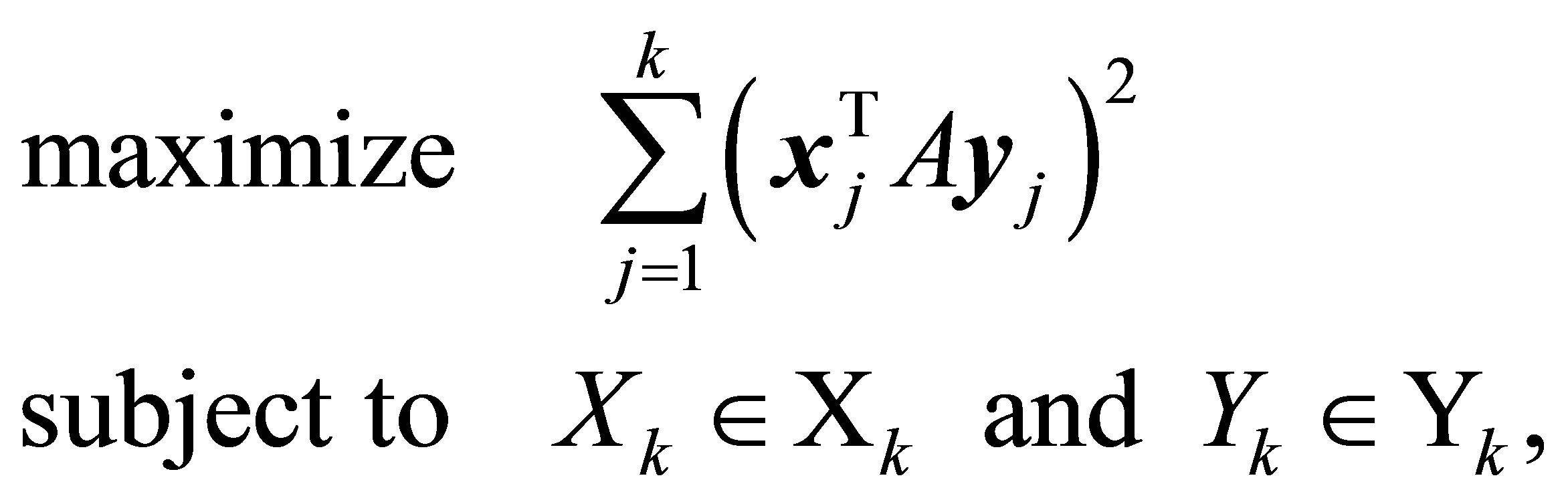 (6.13)
respectively. The SVD matrices  and
and  solve both problems.
Let , denote the singular values of the orthogonal quotients matrix
 . Then, clearly,
 (6.14)
and the Eckart-Young problem (6.12) can be rewritten as
 (6.15)
In the next sections we consider extended problems of this type. The key for solving the extended problems lies in the properties of symmetric orthogonal quotients matrices.
7. The Symmetric Quotients Equality and Ky Fan’s Extremum Principles
Let  be a real
  symmetric matrix with spectral decomposition
 (7.1)
(7.1)
where  is a diagonal
  matrixand
  is an orthogonal
  matrix,
 . It is assumed that the eigenvalues of
  are sorted to satisfy
 (7.2)
(7.2)
Let  be a given
  matrix with orthonormal columns and let
denote the  diagonal matrix which forms the diagonal of
 . Recall that
is invariant under (orthogonal) similarity transformations. Hence by following the proof of (6.1) we obtain the following results.
Theorem 19 (The Symmetric Quotients Equality) Using the above notations,
 (7.3)
(7.3)
and
 (7.4)
(7.4)
where

Note that Theorem 19 remains valid when  is replaced by any real
  matrix. The role of symmetry becomes prominent in problems that attempt to maximize or minimize
 , as considered by Ky Fan [10]. In our notations Ky Fan’s problems have the form
 (7.5
(7.5
and
 (7.6)
(7.6)
The solution of these problems lies in the following well-known properties of symmetric matrices, e.g., [16,30,40].
Theorem 20 (Cauchy Interlace Theorem) Let the  matrix
  be obtained from
  by deleting
  rows and the corresponding
  columns. Let
denote the eigenvalues of . Then
 (7.7)
(7.7)
In particular, when ,
,
 (7.8)
(7.8)

Corollary 21 (Poincaré Separation Theorem) Let  be a given
  matrix with orthonormal columns, and let
  be an orthogonal
  matrix, whose first
  columns are the columns of
 . Then
  is obtained from
  by deleting the last
  rows and the last
  columns. Therefore, since
  has the same eigenvalues as
 , the eigenvalues of
  satisfy (7.7) and (7.8).
Corollary 22 (Ky Fan’s Extremum Principles) Consider the spectral decomposition (7.1)-(7.2) and let the matrix  be constructed from the first k columns of
 . Then
  solves (7.5), giving the optimal value of
 . That is,
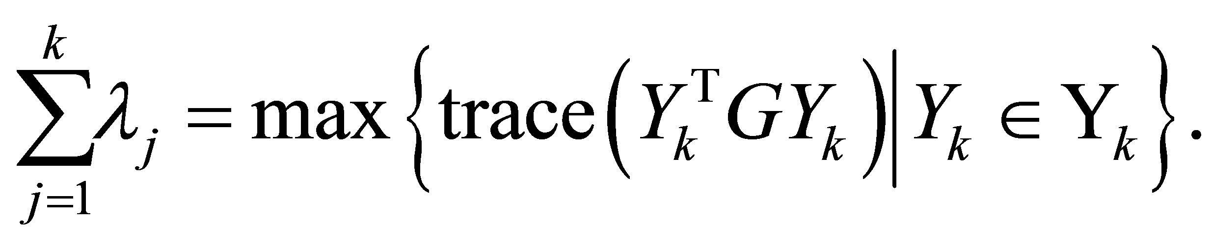 (7.9)
(7.9)
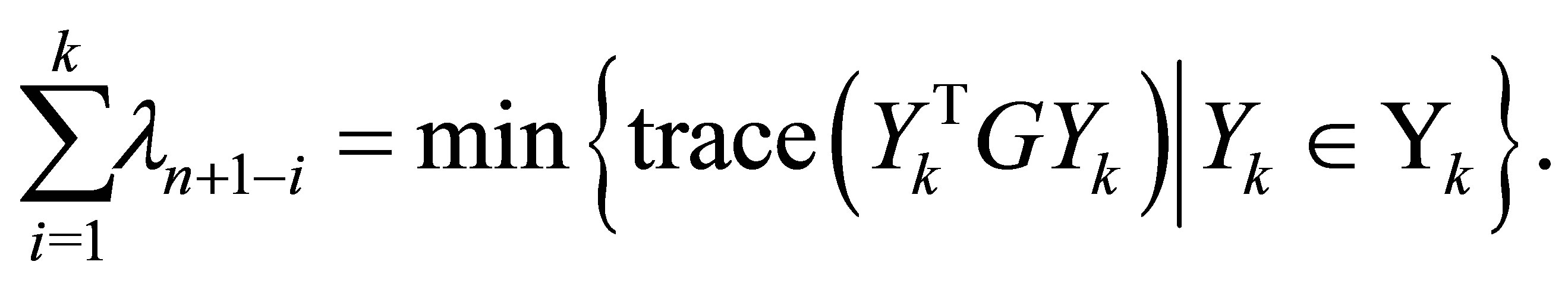
The minimum trace problem (7.6) is solved by the matrix
which is composed of the last  columns of
 . The optimal value of (7.6) is, therefore,
 . That is,
 (7.10)

The symmetric quotients equality (7.3) means that Ky Fan’s problems, (7.5) and (7.6), are equivalent to the problems
 (7.11)
and
 (7.12)
respectively. Note the remarkable similarity between Eckart-Young problems (6.8) and (6.12), and Ky Fan problems (7.11) and (7.5), respectively.
A further insight is gained by considering the case when G is positive semidefinite. In this case the spectral decomposition (7.1)-(7.2) coincides with the SVD of  and the
  matrix
  is also positive semidefinite. Let
 (7.13)
denote the eigenvalues (the singular values) of this matrix. Then here the interlacing relations (7.7) imply majorization relations between the singular values of  and the singular values of the matrices
and . Consequently, for any unitarily invariant norm on
 , the matrix
  solves the problem
 (7.14)
while  solves the problem
 (7.15)
In the next section we move from symmetric orthogonal quotients matrices to rectangular ones. In this case singular values take the role of eigenvalues. Yet, as we shall see, the analogy between the two cases is not always straightforward.
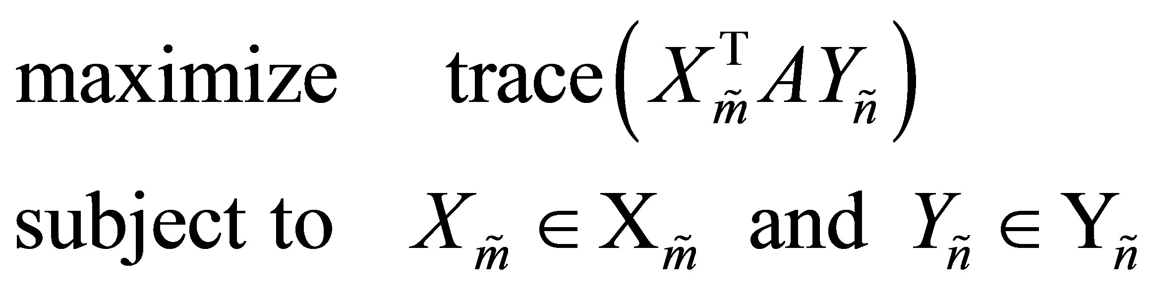
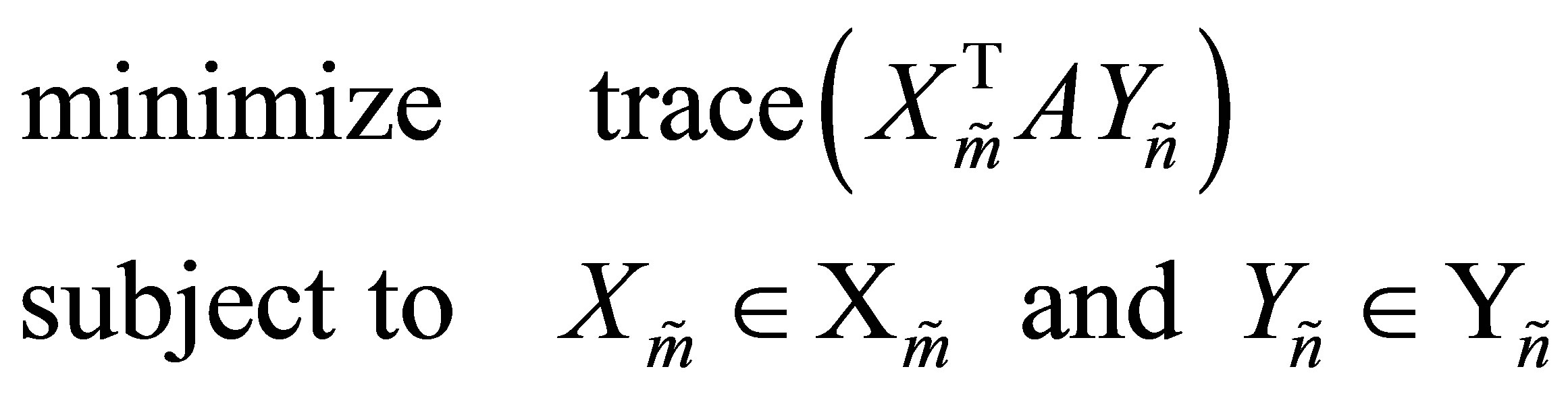
8. Maximizing (Minimizing) Norms of Orthogonal Quotients Matrices
Let us return to consider orthogonal quotient matrices of the form (5.1). Define
and let

denote the singular values of the orthogonal quotients matrix . We shall start by investigating the problems
 (8.1)
(8.1)
and
 (8.2)
(8.2)
where  is a given positive real number,
 . Yet the coming results enable us to handle a larger family of objective functions. Perhaps the more interesting problems of this type occur when
  and
and . In these cases the objective function is reduced to
 (8.3)
(8.3)
and
 (8.4)
(8.4)
respectively. In particular, when  and
and  problem (8.1) coincides with the Eckart-Young problem (6.12). The solution of (8.1) and (8.2) is based on “rectangular” extensions of Theorems 20 and 21. The first theorem is due to Thompson [37]. We outline its proof to clarify its close relation to Cauchy Interlace Theorem.
Theorem 23 (A Rectangular Cauchy Interlace Theorem) Let the  matrix
  be obtained from
  by deleting
  rows and
  columns of
 . That is,
  and
and . Define
and let
denote the singular values of . Then
 (8.5)
(8.5)
Furthermore, the number of positive singular values of  is bounded from below by
where . Consequently
 , and if
  the first
  singular values of
  satisfy the lower bounds
 (8.6)
(8.6)
Proof. The proof is by induction on , where
  is the overall number of deleted rows and columns. For
  there are two cases to consider. Assume first that
  is obtained by deleting one row of
 . Then using Theorem 20 with
  and
and  gives the desired results. The second possibility is that
  is obtained by deleting one column of
 . In this case Theorem 20 is used with
  and
and . Similar arguments enable us to complete the induction step.
Observe that the bounds (8.5) and (8.6) are “strict” in the sense that these bounds can be satisfied as equalities. Take, for example, a diagonal matrix.
Corollary 24 (A Rectangular Poincaré Separation Theorem) Consider the  matrix
 , where
  and
and . Let
. Let
denote the singular values of , where
 . Then
 (8.7)
(8.7)
Furthermore, define  where r = rank (A),
  , and
, and . Then
  and if
  the first
  singular values of
  satisfy the lower bounds
 (8.8)
(8.8)
Proof. Let the matrix  be obtained by completing the columns of
  to be an orthonormal basis of
 . Let the matrix
  be obtained by completing the columns of
  to be an orthonormal basis of
 . Then the
  matrix
  has the same singular values as
 , and
, and  is obtained from
  be deleting the last
  rows and the last
  columns.
Corollary 25 Using the former notations, 
 (8.9)
(8.9)
and
 (8.10)
Furthermore, if  then
then
 (8.11)
and
 (8.12)
Similar inequalities hold when the power function  is replaced by any other real valued function which is increasing in the interval
 .
.
Theorem 26 (A Rectangular Maximum Principle) Let the  matrix
  be constructed from the first
  columns of
 , and let the
  matrix
  be constructed from the first
  columns of
 . (Recall that
  and
and  form the SVD of
 , see (2.1)-(2.8).) Then this pair of matrices solves the maximum problem (8.1), giving the optimal value of
 . That is,
 (8.13)
However, the solution matrices are not necessarily unique.
Proof. The proof is a direct consequence of (8.10) and the fact that  is a diagonal
  matrix whose diagonal entries are
 .
. 
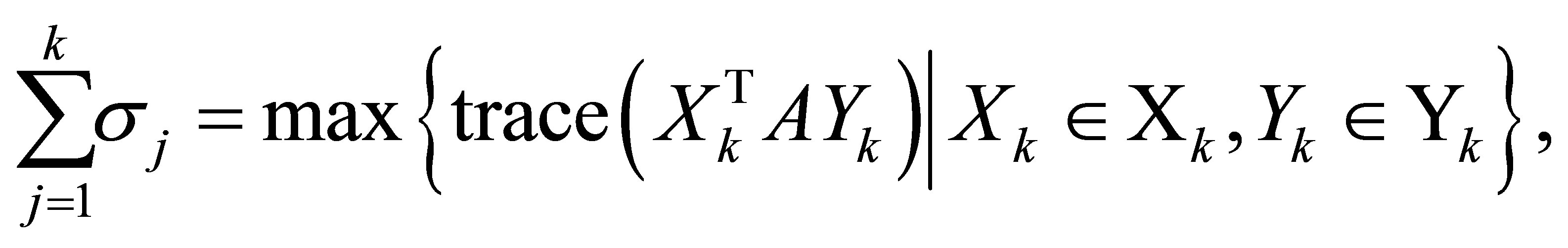
Corollary 27 (A rectangular Ky Fan Maximum Principle) Consider the special case when . In this case
 (8.14)
and the optimal value is attained for the matrices  and
and .
.
Corollary 28 Consider the special case when . In this case
 (8.15)
and the optimal value is attained for the matrices  and
and . Furthermore, if
  then (8.15) is reduced to (6.12). This gives an alternative way to prove the Eckart-Young theorem.
Theorem 29 (A Rectangular Minimum Principle) Let the  matrix
  be obtained from
  by deleting the first
  columns of
 . Let the
  matrix
  be obtained from
  by deleting
 columns in the following way: If
  then
then  is composed from the first
  columns of
 . Otherwise, when
 , the first
  columns of
  are the first
  columns of
 , and the rest columns of
  are the last
  columns of
 . Then the matrices
  and
and  solve the minimum problem (8.2). The optimal value of (8.2) depends on the integer
 . If
. If  the optimal value equals zero. Otherwise, when
 , the optimal value equals
 .
.
Proof. Let the  matrix
  be obtained from the
  identity matrix,
  , by deleting the first
  columns of
 . Then, clearly,
 . Similarly, define
  to be an
  matrix such that
 . That is,
  is obtained from the
  identity matrix by deleting the corresponding columns. With these notations at hand (2.1) implies the equalities
So the matrix  is obtained from
  by deleting the corresponding
  rows and
  columns.
Observe that the remaining nonzero entries of  are the singular values of this matrix. Note also that the rule for deleting rows and columns from
  is aimed to make the size of the remaining nonzero entries as small as possible: The product
  deletes the first
  rows of
 , which contain the largest
  singular values. Then the product
  annihilates the next
  largest singular values. The remaining nonzero entries of
  are, therefore, the smallest that we can get. The number of positive singular values in
  is, clearly,
 . The optimality of our solution stems from (8.8) and (8.12).
Another pair of matrices that solve (8.2) is gained by reversing the order in which we delete rows and columns from : Start by deleting the first
  columns of
 , which contain the
  largest singular values. Then delete the
  rows of
  that contain the next
  largest singular values.
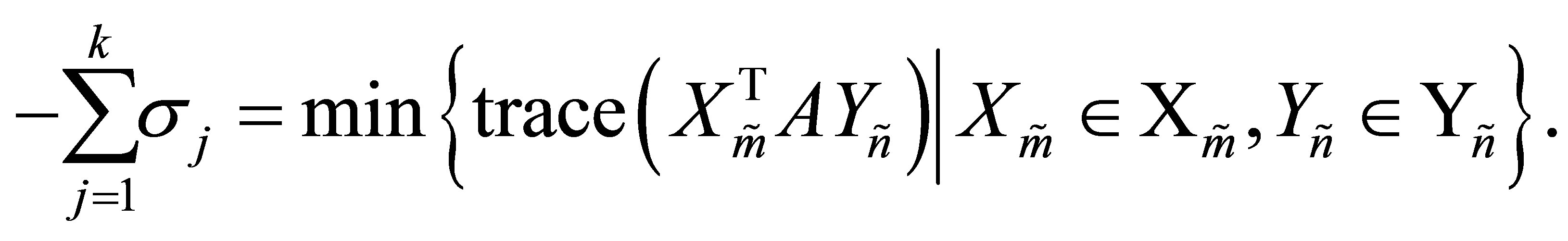
Corollary 30 (A rectangular Ky Fan Minimum Principle) Consider the special case when  and
and . In this case
 (8.16)
and the optimal value is attained for the matrices  and
and .
.
Corollary 31 Consider the special case when  and
and . In this case
 (8.17)
and the optimal value is attained for the matrices  and
and .
.
The next theorem extends our results to arbitrary unitarily invariant norms.
Theorem 32 Let  be a unitarily invariant norm on
 . Then the matrices
  and
and , which solve (8.1), also solve the problem
 (8.18)
Similarly the matrices  and
and , which solve (8.2), also solve the problem
 (8.19)
Proof. From (8.7) we see that the singular values of  are majorized by those of
 . This shows that
 (8.20)
which proves the first claim. Similarly, (8.8) means that the singular values of  are majorized by those of
 . This shows that
 (8.21)
which proves the second claim. 
9. A Minimum-Maximum Equality
The Orthogonal Quotients Equality (6.1) connects the Eckart-Young minimum problem with an equivalent maximum problem. The validity of this equality depends on specific properties of the Frobenius matrix norm. The question raised in this section is whether it is possible to extend this equality to other unitarily invariant matrix norms. In other words, Mirsky’s minimum norm problem (4.22) is related to the maximum norm problem (8.18) The next theorems answer this question when using the Shatten  -norm (2.16) in its power form,
 (9.1)
(9.1)
Theorem 33 (A Minimum-Maximum Equality) Assume that . In this case the power function (9.1) satisfies the equality
 (9.2)
(9.2)
Proof. The optimal value of the minimized term is given by Theorem 9 (Mirsky’s theorem), and this value equals . The optimal value of the other problem is determined by the maximum principle (8.13), and this value equals
 .
. 
If  the power function (9.1) coincides with the trace norm (2.18). In this case (9.2) yields the following elegant result.
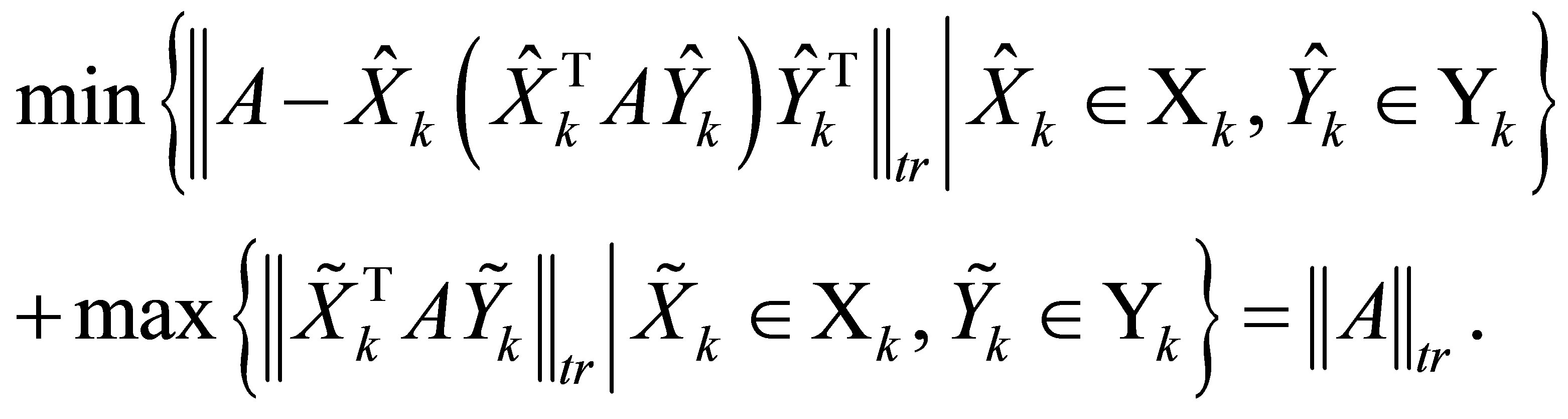 (9.3)
(9.3)
We have seen that Mirsky’s minimization problem (4.22) and the maximum problem (8.18) share a common feature: The optimal values of both problems are obtained for the SVD matrices,  and
and . This observation enables us to extend the minimum-maximum equality to other unitarily invariant norms. Consider, for example, the spectral norm (2.19). In this case (9.3) is replaced with
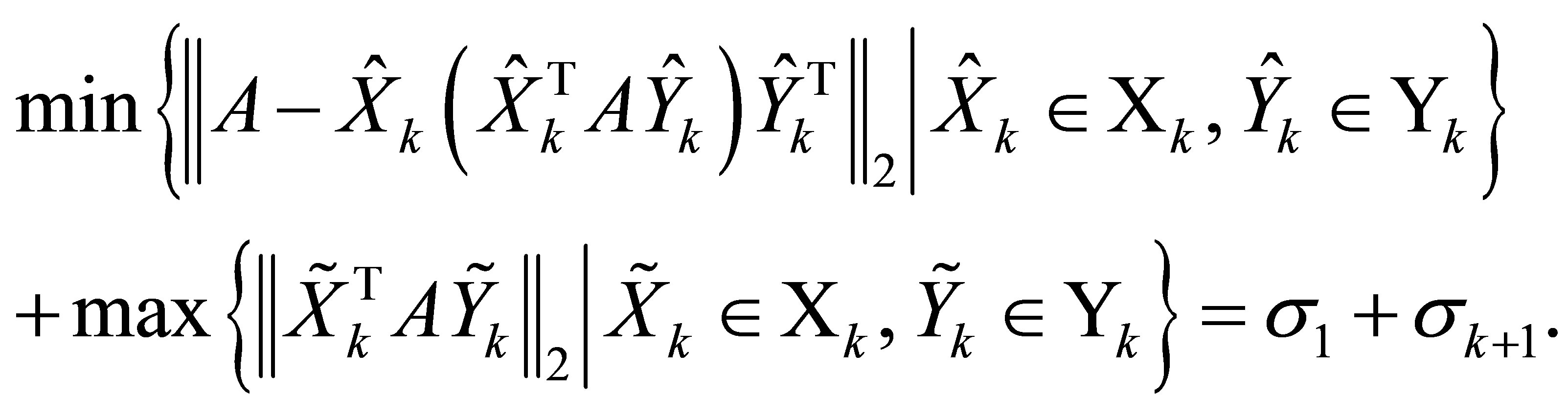 (9.4)
(9.4)
Recall further that the jth columns of the SVD matrices form a pair of singular vectors that correspond to . Indeed, it is this property that ensures the equality in (9.2). This paves the way for another variant of the Orthogonal Quotients Equality.
Theorem 34 Let the matrices  and
and  be composed from pairs of singular vectors of
 . That is,
  , and for
 , the jth columns of these matrices satisfy:
 , and the rectangular quotient
  is a singular value of
 . In this case the power function (9.1) satisfies the equality
 (9.5)
(9.5)
Proof. The term  consists of
  powers of singular values, while the other term consists of the rest
  powers.
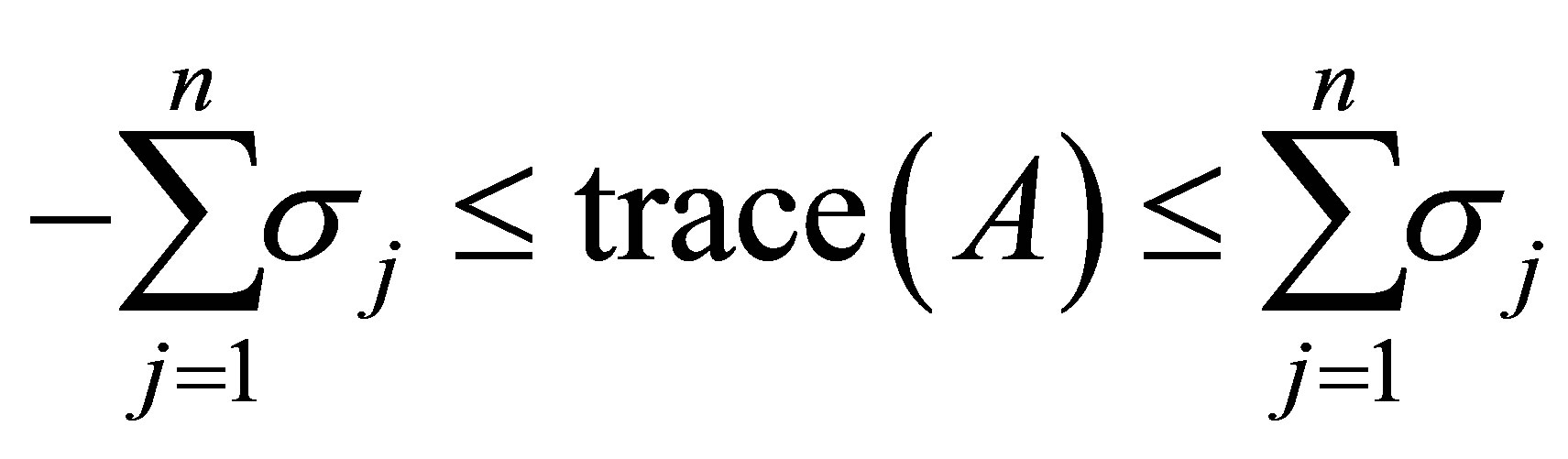
10. Traces of Rectangular Matrices
We have seen that Ky Fan’s extremum principles maximize and minimize traces of symmetric Rayleigh Quotient matrices. In this section we bring analog results in terms of rectangular matrices. For this purpose we define the trace of a rectangular  matrix as
 (10.1)
where . With this definition at hand the new problems to solve are
 (10.2)
and
 (10.3)
Using (2.10) we see that
and
 (10.4)
On the other hand, the matrices  and
and  that solve (8.1) satisfy
 (10.5)
and
 (10.6)
which leads to the following conclusions.
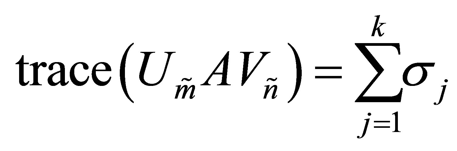
Corollary 35 The matrices  and
and  solve (10.2)
giving the optimal value of . That is,
 (10.7)
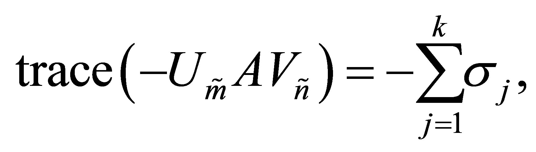
Corollary 36 The matrices  and
and  (or
(or  and
and
 ) solve (10.3) giving the optimal value of
 .
.
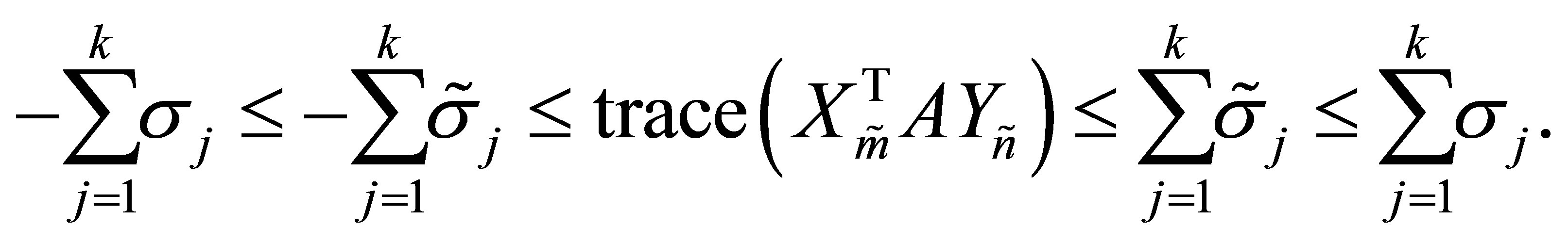
That is
 (10.8)
Finally we note that when  the matrix
  turns to be a square matrix and Corollary 35 is reduced to the following known result.
 (10.9)
e.g., [17, p.~195], [22, p.~515], [24].
11. Products of Eigenvalues versus Products of Singular Values
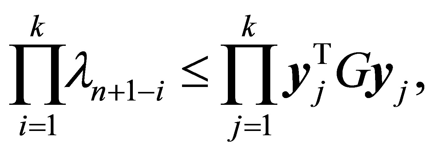
Ky Fan has used his extremum principles (Corollary 22) to derive analog results on determinants of positive semidefinite Rayleigh Quotient matrices (see below). In this section the new principle (Theorem 32) is used to extend these results to Orthogonal Quotient matrices. The interest in these problems stems from the following properties of symmetric matrices. Let G be a real symmetric positive semidefinite  matrix with eigenvalues
Let  be an arbitrary
  matrix with orthonormal columns, and let
denote the eigenvalues of the  matrix
 . Then, clearly,
 (11.1)
while Corollary 21 implies the inequalities
 (11.2)
Let the matrices  and
and  be defined as in Corollary 22. Then the eigenvalues of the matrices
  and
and  are
are
respectively. Hence from (11.2) we see that
 (11.3)
and
 (11.4)
where optimal values are attained for the matrices  and
and , respectively. A further strengthening of (11.4) is gained by applying Hadamard determinant theorem, which says that the determinant of a symmetric positive semidefinite matrix,
  , is smaller than the product of its diagonal entries. That is,
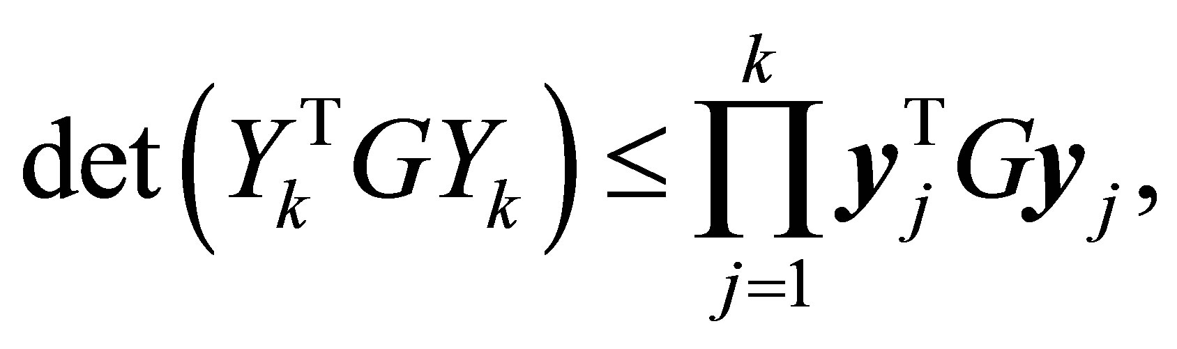 (11.5)
where  denotes the jth column of
 . Combining (11.5) with (11.1) and (11.2) gives the inequality
 (11.6)
for any matrix . Also, as we have seen, equality holds in (11.6) when
 . This brings us to the following observation of Ky Fan [12].
Theorem 37 (Ky Fan)
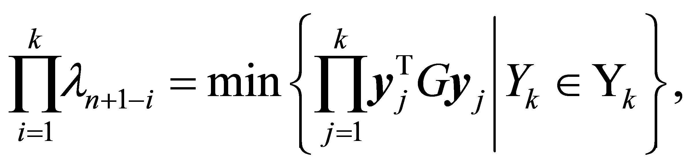 (11.7)
and the optimal value is attained for .
. 
Let us return now to consider rectangular orthogonal quotients matrices. Using the notations of Section 8, the problems that we want to solve are
 (11.8)
and
 (11.9)
(Compare with (8.1) and (8.2), respectively.) Let the matrices  and
and  be defined as in Theorem 26. Using (2.1) one can verify that
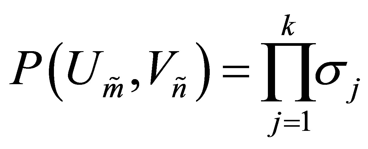 , which is the maximal possible value, see (8.7). This brings us to the following conclusions.
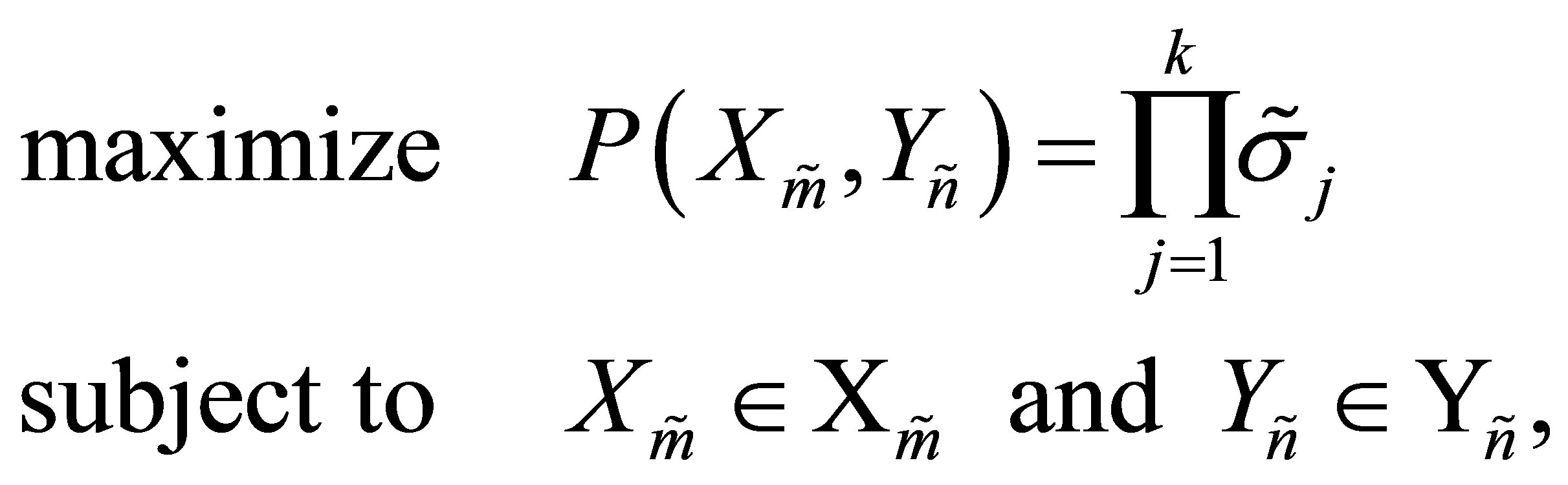
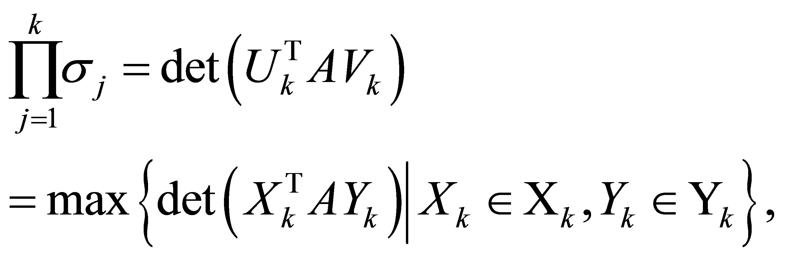
Theorem 38
 (11.10)
and the optimal value is attained for  and
and .
. 
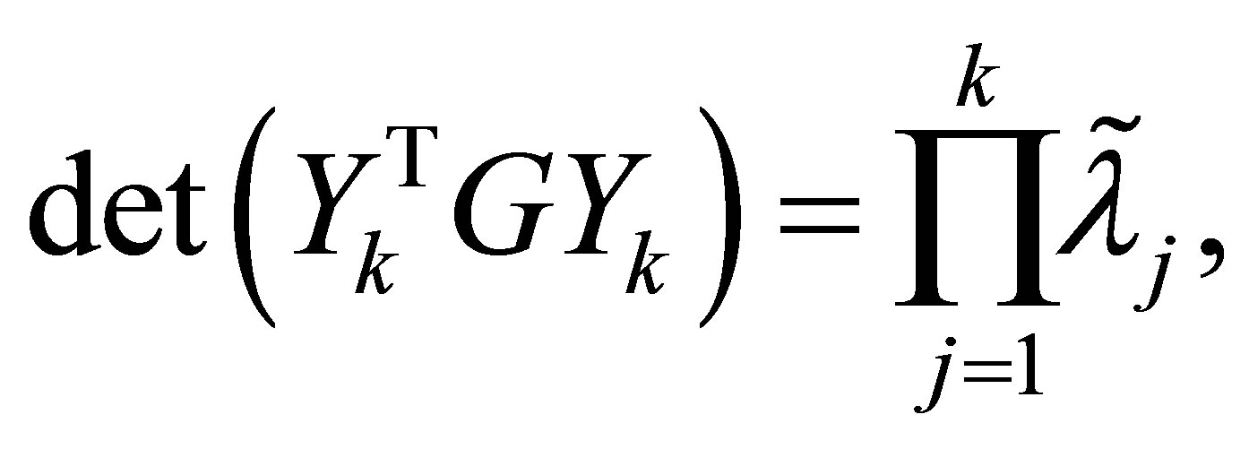
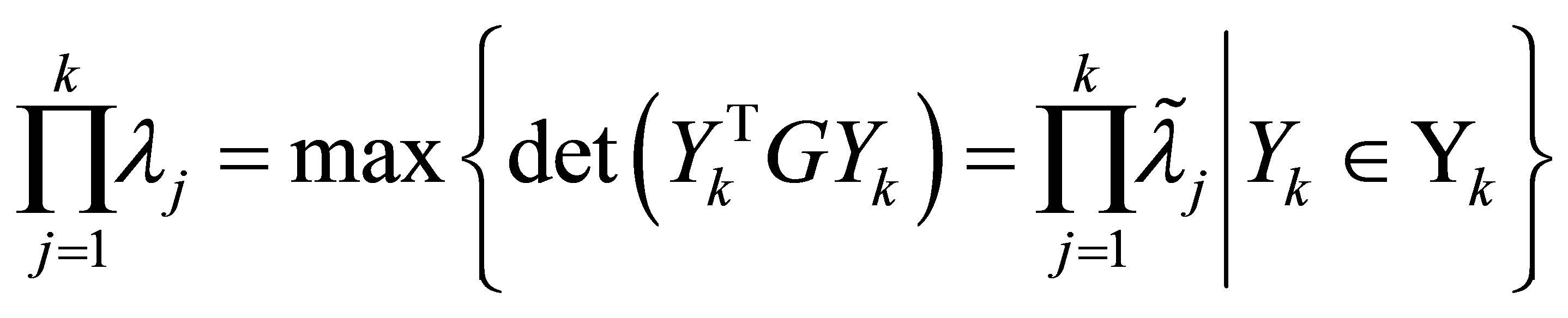
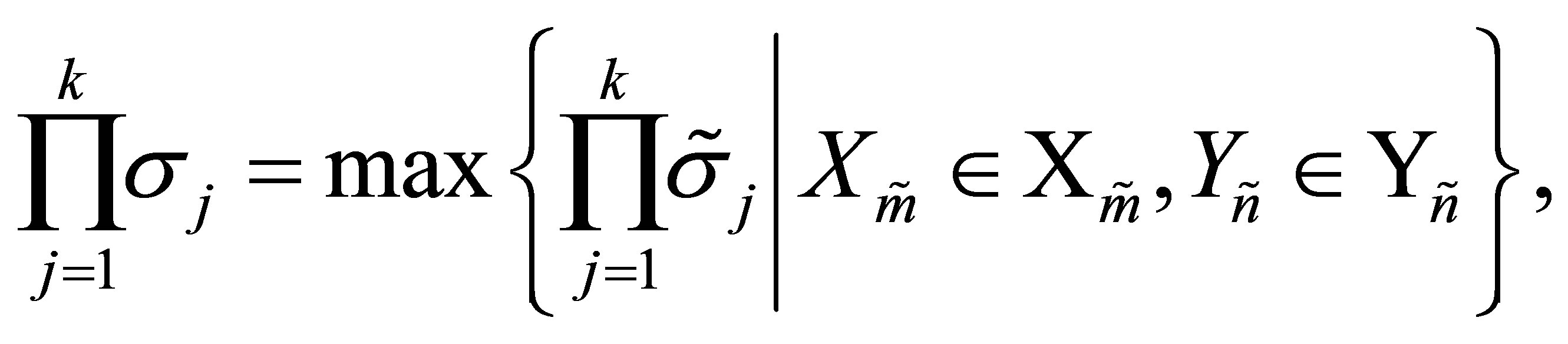
Corollary 39 If  then
then
 (11.11)
where  and
and  are defined in (2.7).
The solution of (11.9) is found by following the notations and the proof of Theorem 29.
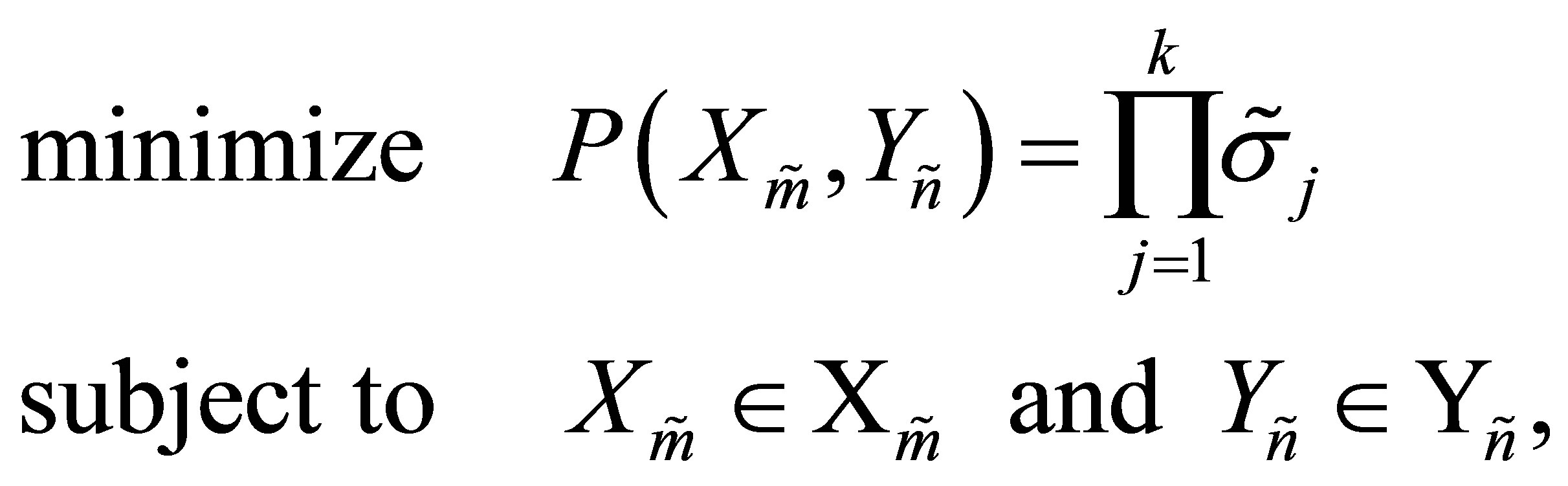
Theorem 40 The matrices  and
and  solve (11.9). The number of positive singular values of the matrix
  is
is . If
. If  then
then
 (11.12)
Otherwise, when ,
,
 (11.13)

Recall that . Hence the equality
  is possible only when r = n. If
  then the equalities
  and r = n imply
  and
and . Otherwise, when
 , the equality
  implies that either
  or
or .
.
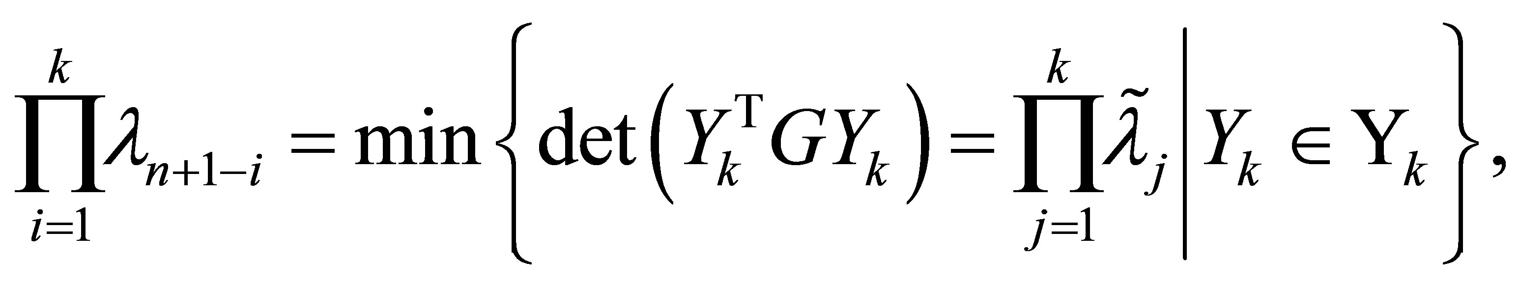
Corollary 41 If  then
then
 (11.14)
12. Concluding Remarks
According to an old adage, the whole can sometimes be much more than the sum of its parts. The Rayleigh-Ritz procedure, the Eckart-Young theorem, and Ky Fan maximum principle are fundamental results that have several applications. The observation that these topics are closely related is new and surprising. It illuminates these issues in a new light.
The extended maximum principle is a powerful tool that has important consequences. In particular we see that both Eckart-Young’s maximum problem and Ky Fan’s maximum problem are special cases of this observation. The minimum-maximum theorem connects the extended maximum problem with Mirsky’s minimum norm problem.
The review provides a second look at results of Ky Fan that consider eigenvalues of symmetric Rayleigh Quotient matrices. It extends these results to “rectangular” versions that consider singular values of Orthogonal Quotients matrices. The proofs illustrate the usefulness of Ky Fan’s dominance theorem. With this theorem at hand Mirsky’s theorem is easily derived from Weyl theorem. Similarly, it helps to establish the extended extremum principle.
REFERENCES
- R. Bhatia, “Matrix Analysis,” Springer, New York, 1997. http://dx.doi.org/10.1007/978-1-4612-0653-8
- X. Chen and W. Li, “On the Rayleigh Quotient for Singular Values,” Journal of Computational Mathematic, Vol. 25, 2007, pp. 512-521.
- A. Dax, “On Extremum Properties of Orthogonal Quotient Matrices,” Linear Algebra and its Applications, Vol. 432, No. 5, 2010, pp. 1234-1257. http://dx.doi.org/10.1016/j.laa.2009.10.034
- J. W. Demmel, “Applied Numerical Linear Algebra,” SIAM, Philadelphia, 1997. http://dx.doi.org/10.1137/1.9781611971446
- G. Eckart and G. Young, “The Approximation of One Matrix by Another of Lower Rank,” Psychometrika, Vol. 1, No. 3, 1936, pp. 211-218. http://dx.doi.org/10.1007/BF02288367
- A. Edelman, T. Arias and S. Smith, “The Geometry of Algorithms with Orthogonality Constraints,” The SIAM Journal on Matrix Analysis and Applications, Vol. 20, No. 2, 1998, pp. 303-353. http://dx.doi.org/10.1137/S0895479895290954
- A. Edelman and S. Smith, “On Conjugate Gradient-Like Methods for Eigen-Like Problems,” BIT Numerical Mathematics, Vol. 36, No. 3, 1996, pp. 494-508. http://dx.doi.org/10.1007/BF01731929
- L. Elden, “Matrix Methods in Data Mining and Pattern Recognition,” SIAM, Philadelphia, 2007. http://dx.doi.org/10.1137/1.9780898718867
- L. Elden and H. Park, “A Procrust S Problem on the Stiefel Manifold,” Technical Report, Department of Mathematics, Linköping University, Linköping, 1997.
- K. Fan, “On a theorem of Weyl Concerning Eigenvalues of Linear Transformations I,” Proceedings of the National Academy of Sciences, USA, Vol. 35, No. 11, 1949, pp. 652-655. http://dx.doi.org/10.1073/pnas.35.11.652
- K. Fan, “Maximum Properties and Inequalities for the Eigenvalues of Completely Continuous Operators,” Proceedings of the National Academy of Sciences, USA, Vol. 37, No. 11, 1951, pp. 760-766. http://dx.doi.org/10.1073/pnas.37.11.760
- K. Fan, “A Minimum Property of the Eigenvalues of a Hermitian Transformation,” The American Mathematical Monthly, Vol. 60, No. 1, 1953, pp. 48-50. http://dx.doi.org/10.2307/2306486
- E. Fischer, “Concerning Quadratic Forms with Real Coefficients,” Monatshefte für Mathematik und Physik, Vol. 16, 1906, pp. 234-249.
- G. H. Golub and C. Van Loan, “An Analysis of the Total Least Squares Problem,” SIAM Journal on Numerical Analysis, Vol. 17, No. 6, 1980, pp. 883-893. http://dx.doi.org/10.1137/0717073
- G. H. Golub and C. F. Van Loan, “Matrix Computations,” Johns Hopkins University Press, Baltimore, 1983.
- R. A. Horn and C. R. Johnson, “Matrix Analysis,” Cambridge University Press, 1985. http://dx.doi.org/10.1017/CBO9780511810817
- R. A. Horn and C. R. Johnson, “Topics in Matrix Analysis,” Cambridge University Press, Cambridge, 1991. http://dx.doi.org/10.1017/CBO9780511840371
- R. M. Johnson, “On a Theorem Stated by Eckart and Young,” Psychometrica, Vol. 28, No. 3, 1963, pp. 259- 263. http://dx.doi.org/10.1007/BF02289573
- W. Kahan, B. N. Parlett and E. Jiang, “Residual Bounds on Approximate Eigensystems of Nonnormal Matrices,” SIAM Journal on Numerical Analysis, Vol. 19, No. 3, 1982, pp. 470-484.
- R.-C. Li, “On Eigenvalues of a Rayleigh Quotient Matrix,” Linear Algebra and Its Applications, Vol. 169, 1992, pp. 249-255. http://dx.doi.org/10.1016/0024-3795(92)90181-9
- X. G. Liu, “On Rayleigh Quotient Theory for the Eigenproblem and the Singular Value Problem,” Journal of Computational Mathematics, Supplementary Issue, 1992, pp. 216-224.
- A. W. Marshall and I. Olkin, “Inequalities: Theory of Majorization and Its Applications,” Academic Press, New York, 1979.
- L. Mirsky, “Symmetric Gauge Functions and Unitarily Invariant Norms,” Quarterly Journal of Mathematics, Vol. 11, No. 1, 1960, pp. 50-59. http://dx.doi.org/10.1093/qmath/11.1.50
- J. von Neumann, “Some Matrix-Inequalities and Metrization of Matrix-Space,” Tomsk. Univ. Rev., Vol. 1, 1937, pp. 286-300. (In: A. H. Taub, Ed., John von Neumann Collected Works, Vol. IV, Pergamon, Oxford, 1962, pp. 205-218.)
- D. P. O’Leary and G. W. Stewart, “On the Convergence of a new Rayleigh Quotient Method with Applications to Large Eigenproblems,” TR-97-74, Institute for Advanced Computer Studies, University of Maryland, College Park, 1997.
- A. M. Ostrowski, “On the Convergence of the Rayleigh Quotient Iteration for the Computation of the Characteristic Roots and Vectors. III (Generalized Rayleigh Quotient and Characteristic Roots with Linear Elementary Divisors,” Archive for Rational Mechanics and Analysis, Vol. 3, No. 1, 1959, pp. 325-340. http://dx.doi.org/10.1007/BF00284184
- A. M. Ostrowski, “On the Convergence of the Rayleigh Quotient Iteration for the Computation of the Characteristic Roots and Vectors. IV (generalized Rayleigh Quotient for Nonlinear Elementary Divisors,” Archive for Rational Mechanics and Analysis, Vol. 3, No. 1, 1959, pp. 341-347. http://dx.doi.org/10.1007/BF00284185
- M. L. Overton and R. S. Womersley, “On the Sum of the Largest Eigenvalues of a Symmetric Matrix,” SIAM Journal on Numerical Analysis, Vol. 13, No. 1, 1992, pp. 41- 45. http://dx.doi.org/10.1137/0613006
- B. N. Parlett, “The Rayleigh Quotient Iteration and Some Generalizations for Nonnormal Matrices,” Mathematics of Computation, Vol. 28, No. 127, 1974, pp. 679-693. http://dx.doi.org/10.1090/S0025-5718-1974-0405823-3
- B. N. Parlett, “The Symmetric Eigenvalue Problem,” Prentice-Hall, Englewood Cliffs, 1980.
- E. Schmidt, “Zur Theorie der Linearen und Nichtlinearen Integralgleichungen. I Teil. Entwicklung Willkürlichen Funktionen nach System Vorgeschriebener,” Mathematische Annalen, Vol. 63, No. 4, 1907, pp. 433-476. http://dx.doi.org/10.1007/BF01449770
- G. W. Stewart, “Two Simple Residual Bounds for the Eigenvalues of Hermitian Matrices,” SIAM Journal on Matrix Analysis and Applications, Vol. 12, No. 2, 1991, pp. 205-208. http://dx.doi.org/10.1137/0612016
- G. W. Stewart, “Matrix Algorithms,” Vol. I: Basic Decompositions, SIAM, Philadelphia, 1998.
- G. W. Stewart, “Matrix Algorithms,” Vol. II: Eigensystems, SIAM, Philadelphia, 2001.
- E. Stiefel, “Richtungsfelder und Fernparallelismus in nDimensionalen Mannigfaltigkeiten,” Commentarii Mathematici Helvetici, Vol. 8, No. 1, 1935-1936, pp. 305-353.
- J. G. Sun, “Eigenvalues of Rayleigh Quotient Matrices,” Numerische Mathematik, Vol. 59, No. 1, 1991, pp. 603- 614. http://dx.doi.org/10.1007/BF01385798
- R. C. Thompson, “Principal Submatrices IX: Interlacing Inequalities for Singular Values of Submatrices,” Linear Algebra and its Applications, Vol. 5, 1972, pp. 1-12.
- R. C. Thompson, “The Behavior of Eigenvalues and Singular Values under Perturbations of Restricted Rank,” Linear Algebra and Its Applications, Vol. 13, No. 1-2, 1976, pp. 69-78. http://dx.doi.org/10.1016/0024-3795(76)90044-6
- H. Weyl, “Das Asymptotische Verteilungsgesetz der Eigenwerte Linearer Partieller Differentialgleichungen (Mit Einer Anwendung auf die Theorie der Hohlraumstrahlung,” Mathematische Annalen, Vol. 71, No. 4, 1912, pp. 441-479. http://dx.doi.org/10.1007/BF01456804
- J. H. Wilkinson, “The Algebraic Eigenvalue Problem,” Clarendon Press, Oxford, 1965.
- F. Zhang, “Matrix Theory: Basic Results and Techniques,” Springer-Verlag, New York, 1999. http://dx.doi.org/10.1007/978-1-4757-5797-2