World Journal of Mechanics
Vol.4 No.2(2014), Article ID:42981,10 pages DOI:10.4236/wjm.2014.42006
A New Class of Vector Padé Approximants in the Asymptotic Numerical Method: Application in Nonlinear 2D Elasticity
Laboratoire d’Ingénierie et Matériaux LIMAT, Faculté des Sciences Ben M’Sik, Université Hassan II Mohammedia - Casablanca, Casablanca, Maroc
Email: abdellah.hamdaoui@univh2m.ac.ma, hihi_rachida@hotmail.com, b.braikat@gmail.com, no_tounsi@live.fr, noureddine.damil@univh2m.ma
Received November 14, 2013; revised December 16, 2013; accepted January 12, 2014
ABSTRACT
The Asymptotic Numerical Method (ANM) is a family of algorithms for path following problems, where each step is based on the computation of truncated vector series [1]. The Vector Padé approximants were introduced in the ANM to improve the domain of validity of vector series and to reduce the number of steps needed to obtain the entire solution path [1,2]. In this paper and in the framework of the ANM, we define and build a new type of Vector Padé approximant from a truncated vector series by extending the definition of the Padé approximant of a scalar series without any orthonormalization procedure. By this way, we define a new class of Vector Padé approximants which can be used to extend the domain of validity in the ANM algorithms. There is a connection between this type of Vector Padé approximant and Vector Padé type approximant introduced in [3, 4]. We show also that the Vector Padé approximants introduced in the previous works [1,2], are special cases of this class. Applications in 2D nonlinear elasticity are presented.
Keywords:Vector Padé Approximants; Asymptotic Numerical Method; Nonlinear Elasticity
1. Introduction
Many engineering problems can be reduced to solving nonlinear problems depending on a control parameter λ. These problems are written in general form:
 (1)
(1)
where  is the unknown vector of
 ,
,  is a vector function with values in
  assumed to be sufficiently regular with respect to its arguments
  and
and .
.
The Asymptotic Numerical Method (ANM) [1,2] is a family of algorithms for path following problems. The principle is simply to expand the unknown  of the nonlinear problem (1) in power series with respect to a path parameter “a”:
 (2)
(2)
where ,
,  ,
,
 is a known and regular solution corresponding to
  and
and  is the truncated order of the series. The interval of validity
  is deduced from the computation of the truncated vector series (2). So, the step lengths are computed a posteriori by the following estimation of
 , which have been proposed in [1]:
 (3)
(3)
where  is a given tolerance parameter and
  indicates a standard norm. The step lengths depend on the definition of the path parameter “a” and we must add an auxiliary equation to define this parameter [1]. By using the evaluation of the series at
 , we obtain a new starting point and define, in this way, the ANM continuation procedure. This continuation method has been proved to be an efficient method to compute the solution of nonlinear partial differential equations [1,2].
The Vector Padé approximants were introduced in the ANM to improve the domain of validity  of vector series (polynomial) representation [2]. In order to extend the domain of validity of the representation (2) and to reduce the number of steps needed to obtain the entire solution path, in [2], a rational approximation, called Padé approximant [5-8], has been used. In [2], the representation (2) has been rewritten in an orthonormal basis built up from the basis
  generated by the ANM and a strategy to use Vector Padé approximants has been applied. This has been used in various fields [1,9]. But this strategy had the disadvantage to generate a great number of poles inside the domain of validity. An alternative, presented in [1], is to use Vector Padé approximants with a common denominator, called simultaneous Padé approximants [7,8]. The orthonormalization can be done according to the procedure of Gram-Schmidt or modified Gram-Schmidt or iterative Gram-Schmidt [1], or as it will be presented in this paper for the first time by using the Householder method.
Many applications in structural mechanics (for instance nonlinear elasticity and contact), [1,2] have established that Vector Padé approximants with a common denominator can reduce the number of poles and permit to obtain more regular solutions. By using this rational representation in a continuation procedure, the number of steps to obtain the entire solution path has been reduced [10]. The Vector Padé approximants have also been considered to accelerate the convergence of high order iterative algorithms for linear or nonlinear [1] problems.
The aim of this paper is to discuss some techniques to define new Vector Padé approximants in the framework of the ANM and to show that their utilization can improve clearly the classical Vector Padé representation.
In the second part, we propose a new type of Vector Padé approximant which can be directly defined from the vector series (1) by extending the definition of the Padé approximant of a scalar series [5,8] and without any orthonormalization procedure. By this way, we show that a family of Vector Padé approximants is possible. There is a connection between this type of Vector Padé approximant and Vector Padé type introduced in [3,4]. We show also that the Vector Padé approximant introduced in the previous works [1,2] are special cases of this class.
All the approximants are applied on some examples from nonlinear two-dimensional elasticity which are presented and analyzed in the third part. Among this family of Vector Padé approximant, we show on numerical examples, that there are some approximants which increase the range of validity  and thus reduce the number of steps necessary for the calculation of solutions. To illustrate this, three numerical tests in two-dimensional nonlinear elasticity are considered: traction of an elastic plate, bending of an elastic plate and bending of an elastic arch. These structures are discretized by the conventional finite element method using a CST element [11].
2. Definition and Construction of a New Type of Vector Padé Approximant
In this Section, we will give the definition and the construction of a new type of vector Padé approximants.
2.1. Definition
A Vector Padé approximant of a vector function  from
from  to
to  is a “Vector fraction” whose Taylor expansion at a given order, coincides with the vector functions one. More precisely, the Vector Padé approximant
  is the ”vector rational fraction” of the form:
 (4)
(4)
where  matrices are of dimension
  and
and  vectors are in
 . This ”vector rational fraction”
  admits the same Taylor expansion than the vector function
  up to order
  (
(![]() are integers).
are integers).
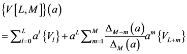
The aim of this paper is to define Vector Padé approximant  following the same ideas as in the scalar case:
 (5)
(5)
where  is a vector whose components are polynomials of degree
  and
and  is a matrix whose elements are polynomials of degree
 ,
,  , which are as
 (6)
(6)
The vector ”polynomial” , and the matrix ”polynomial”
  are derived from the vector function
  from the condition:
 (7)
(7)
In Appendix 1, we show that the  matrices
 ,
,  in (6) are solutions of the following linear system:
 (8)
(8)
and the  vectors
 ,
, ![]() , given in (6) are derived from the following relationships:
, given in (6) are derived from the following relationships:
 (9)
(9)
The system (8) can be written in the following matrix form (see Appendix 1)
 (10)
(10)
It may be noted that if the terms of the series in Equations (6) are scalar, we find exactly the system defining the scalar Padé approximant in [8]. Note also that in the case where the matrix  is of the form
 , where
  is a polynomial of degree
  and
and  is the unit matrix, we find the definition of Vector Padé type approximant
  introduced in [3,4]. The new definition also allows finding Vector Padé approximants classically used in the ANM algorithm [1]. Recall that classically in the ANM algorithm, the Padé approximant associated with the vector series is constructed by replacing each scalar series components by a scalar Padé approximant, or by replacing the scalar polynomials, which appear after orthonormalization of the vector basis, by scalar Padé approximants with the same denominator [1]. These cases will be found in the following paragraph.
2.2. Construction of Some Vector Padé Approximants
The construction of the new type of Vector Padé approximants requires the solution of the matrix system (10) verified by the matrices . This system allows, in general, an infinite number of solutions. Indeed, a family of solutions of (10) can be obtained in the following general form:

where  is any rectangular matrix having
rows and  columns. We easily check that the product of the matrix
  by the formula of the matrix solution
  gives the matrix
 . Note that in this family of solutions, the matrix
  is invertible because the row vectors of
  are assumed linearly independent.
Note that in the scalar case, the matrix  in the system (10) is a square matrix. Therefore, the system (10) has a unique solution if the matrix
  is invertible.
According to the definition of the Vector Padé approximant (4), the construction of this new type of Vector Padé approximant usually requires high computational cost due to the fact that for each value of a, we need to calculate the inverse of the matrix  defining the Vector Padé approximant in (4). However, there are situations in which we can explicitly calculate the inverse of the matrix
  for all values of a.
For example, if we look for matrices,  ,
,  in diagonal form,
  , where
  are real, then we find that the components of the Vector Padé approximant
  are given by the following formula (see Appendix 2 ):
 (11)
(11)
It corresponds to the Vector Padé approximant that would be built from the scalar Padé approximant corresponding to each component of the vector  as it was pointed in ANM framework [1].
Another choice of the form of the matrices ,
,  , based initially on the orthonormalisation of vectors
 ,
, ![]() (see Appendix 2), leads to the following Vector Padé approximants:
(see Appendix 2), leads to the following Vector Padé approximants:
 (12)
(12)
where the polynomial  in (12) depends on the coefficients
 , which are calculated from the orthonormalization procedures of the vectors
 ,
,![]() :
:

In Appendix 2, we show that the scalars  are arbitrary and so we can use the new expression of the Vector Padé approximant (12) giving the coefficients
  any values. Note that for
 , the Vector Padé approximant reduces to:
 (13)
(13)
We thus find the Vector Padé approximant (13) introduced in the work of the ANM algorithms [1,2] where the coefficients  are determined from a Gram-Schmidt orthonormalisation of the vectors
  of the series (2).
Therefore, we constructed a new family of Vector Padé approximants given by Equation (12) or (13) without any condition on the coefficients . In the following numerical applications, we demonstrate that there are choices for these coefficients for which the range of validity is larger than in the cases conventionally used.
2.3. Continuation Procedure
The representations (2) or (13) permit to compute only a part of the solution path of the nonlinear problem (1). To obtain the entire solution path, Cochelin [1] proposed a continuation procedure for the vector series representation (2) based on the criterion (3) which gives an evaluation of the domain of validity of the polynomial representation. Once the determination of the domain of validity is done, by the computation of the radius of validity  for a fixed tolerance ε , the vector series representation (2) can be applied in a continuation procedure to obtain the entire solution path step by step.
To introduce the vector Padé representation in a continuation algorithm, Elhage et al. [10] proposed another criterion defined by:

which gives an evaluation of the radius of validity  of the rational representation for a fixed tolerance
![]() , by using a dichotomy process. We shall use the same criterion to introduce the proposed Vector Padé representations (13) in a continuation process.
, by using a dichotomy process. We shall use the same criterion to introduce the proposed Vector Padé representations (13) in a continuation process.
3. Numerical Applications
The numerical robustness of the approximate solutions obtained by the vector series representation (2) and by the new family of Vector Padé representation (12) is discussed on the basis of tests emanating from plane stress two-dimensional nonlinear elasticity analysis. The studied structure is discretized using a classical CST finite element [11] and is subjected to a loading proportional to a control parameter . We seek the solution of this problem by representing the control parameter
  as a function of displacement. The quality of ANM steps is evaluated from load-deflection curves and residual deflection curves and the main criterion is the step lengths.
More precisely, we plot the load-displacement curves with three ANM steps. Three calculations are carried out:
• the first calculation will be made using ANM continuation with a series representation (2)• the second calculation will be made using ANM continuation with classical Vector Padé representation (12), the coefficients  are derived from an orthonormalization procedure, here by the method of Householder• the third calculation will be made using ANM continuation with the proposed Vector Padé representation (12) but this time the coefficients
  are arbitrary.
The performance of the three calculations are compared in terms of the step lengths of the three ANM continuations, the quality of the solutions is given by the residual curves.
3.1. Bending of a Plate
The first numerical example concerns the bending of a plate; see Figure 1, the plate has a length of 100 mm and a width of 10 mm. The plate is clamped on the left side and subjected to a bending force proportional to a control parameter  on the other end. Material characteristics are: Young’s modulus E = 10,000 MPa, Poisson’s ratio
 . The plate was discretized using 41 nodes along the length and six nodes along the width; a total of 400 elements and 492 degrees of freedom is used.
In Figure 1, we represent the response curves obtained by the ANM continuation giving the loading parameter  as a function of the displacement
  at the node 246. We plotted the load-displacement curves using three ANM steps for the three calculations and for three choices of the truncation order: 10, 15 and 20. In Figure 2, for the three calculations, we represent the residual curve giving the logarithm of the norm of the residual
  as a function of displacement at node 246.
The first calculation, ANM continuation with series representation (2), at orders 10, 15 and 20, shows that the step length increases with the truncation order. Three steps at order 20, allow obtaining the curve until a displacement equal to 62 mm with accuracy of the order of 10−5. This result is classical in the works of ANM algorithm [1], the increase of the order increases the step length.
The second calculation, ANM continuation with classical Padé representation, at orders 10, 15 and 20, shows
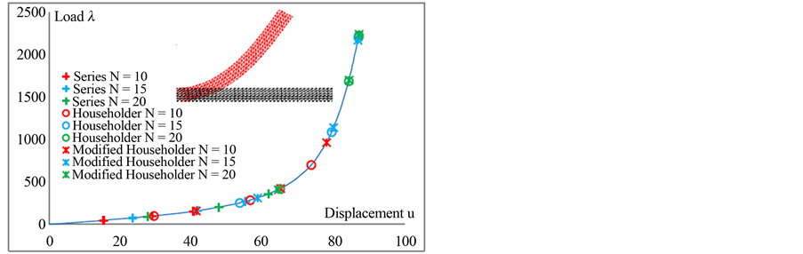
Figure 1. Bending of a plate, load-displacement curve,  versus displacement at node 246 for the three types of calculation for truncation orders 10, 15 and 20.
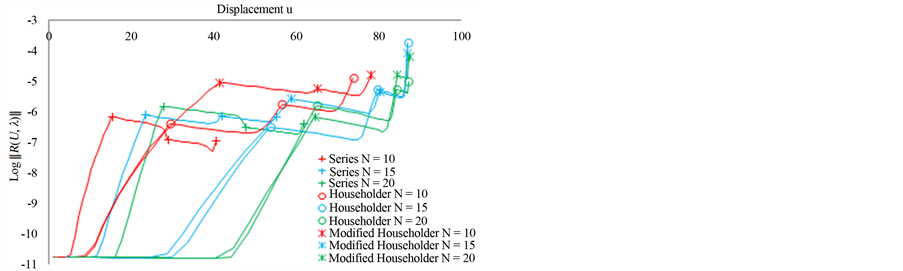
Figure 2. Bending of a plate, residual curve,  as a function of the displacement u at node 246 for the three types of calculation for orders 10, 15 and 20.
that the step lengths are greater than the first calculation using series representation. Three steps with ANM Padé representation at order 10 allows obtaining the curve until a displacement equal to 73 mm with a good quality as can be seen on the residual curve of Figure 2.
For this second calculation, the results obtained by using the Householder orthonormalisation method are compared with those obtained by using Gram-Schmidt orthonormalization in Figure 3. In all our numerical experiments, the Householder orthonormalization method seems more effective than Gram-Schmidt orthonormalizations procedure. We will use in the following, the method of Householder.
The third calculation, ANM continuation with the proposed Vector Padé representation (12) the coefficients being arbitrary, is performed by using the orders 10, 15 and 20. We carried out the calculations by slightly modifying the values of the coefficients , calculated by the method of Householder for each order. All the values of the coefficients were increased by a value equal to 0.1.
This first test was very successful. Indeed, it shows that an arbitrary choice of the coefficients  can give good results as can be seen in the response curve in Figure 1 and the residual curve in Figure 2. Three steps with the proposed ANM Padé representation at order 10 allows obtaining the curve until a displacement equal to 78 mm with a good quality as can be seen on the residual curve of Figure 2.
3.2. Bending of an Elastic Arch
For the second numerical experiment, we chose the example of the bending of an elastic arch, see Figure 4, of radius R = 2540 mm, width of 15 mm and an angle of 0:1 rad. The arch is clamped at both ends and is subjected to a bending force proportional to a control parameter  at its middle. Material characteristics are: Young’s modulus E = 10,000 MPa, Poisson’s ratio
 . The arch
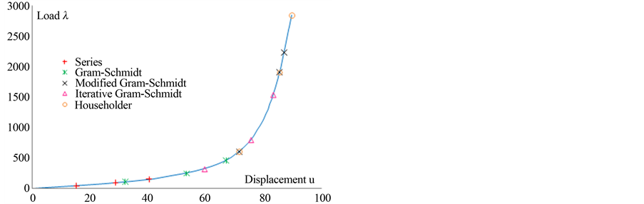
Figure 3. Bending of a plate, load-displacement curve,  as a function of the displacement u at node 246. Comparison of ANM continuation using Vector Padé representation for four processes of orthonormalisations: Gram-Schmidt, modified Gram-Schmidt, iterative Gram-Schmidt and Householder at order 29.
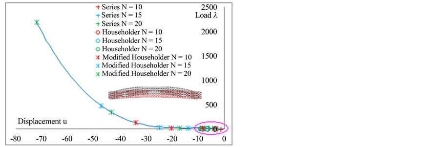
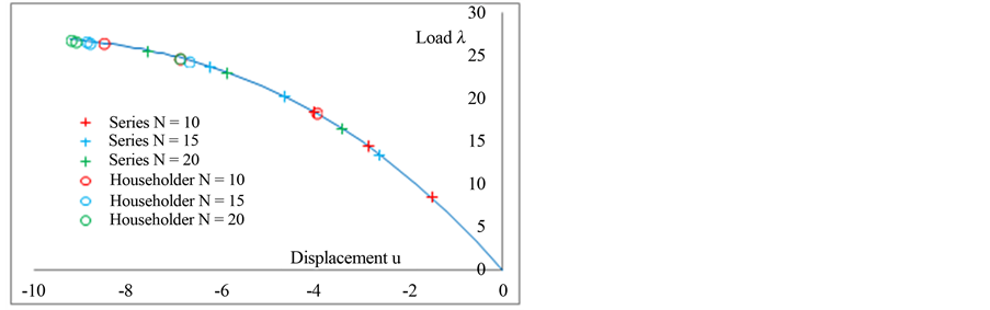
Figure 4. Bending of an elastic arch, load-displacement curve,  versus the displacement u at node 152 for the three types of calculation for truncation orders 10, 15 and 20.
was discretized using 41 nodes along the radius and five nodes along the width; a total of 320 elements and 410 degrees of freedom is used.
We represent in Figure 4, the response curve obtained by ANM algorithms giving the loading parameter  as a function of displacement u at node 105. Residual curves are given in Figure 5.
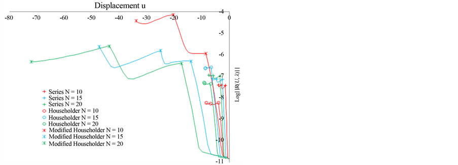
Figure 5. Bending of an elastic arch, residual curve,  as a function of the displacement u for the three types of calculation for orders 10, 15 and 20.
The results obtained by respectively the first calculation, ANM continuation by using series representation (2) at orders 10, 15 and 20, the second calculation, ANM continuation by using classical vector Padé approximation at orders 10, 15 and 20, the coefficients  are derived from the Householder orthonormalisation method, and the third calculation, ANM continuation using the proposed Vector Padé representation (12) at orders 10, 15 and 20, the values of the coefficients
  were increased by a value equal to 0.1 are reported on Figures 4 and 5.
Three steps with the proposed ANM Padé representation at order 20 allows obtaining the curve until a displacement equal to −72 mm with a good quality as can be seen on the residual curve of Figure 5. While three steps with the classical ANM Padé representation at order 20 allows obtaining the curve until a displacement equal to −10 mm and the three steps with the ANM with the series representation at order 20 allows obtaining the curve until a displacement equal to −8 mm, see Figure 5.
This second numerical test confirms that an arbitrary choice of the coefficients  can give very good results as we can see from the response curve in Figure 4 and the residual curve of Figure 5.
3.3. Traction of an Elastic Plate
For the third numerical experiment, we consider the traction of an elastic plate; see Figure 6, the plate has a length of 100 mm and a width of 25 mm. The plate is clamped on the left side and subjected to a tensile force, on the other end, proportional to a control parameter . Material characteristics are: Young’s modulus E = 10,000 MPa, Poisson’s ratio
 . The plate was discretized using 41 nodes along the length and six nodes along the width; a total of 400 elements and 492 degrees of freedom is used.
We represent in Figure 6, the response curves obtained using three methods of ANM continuation at orders 10, 15 and 20 used in the previous cases. The residual curves are given in Figure 7. This test confirms the results obtained in the first two numerical tests. In particular, this example also shows that an arbitrary choice of the coefficients  can give very good results as can be seen on the response curve, Figure 6, and the residual curve, Figure 7.
4. Conclusion
In this work, we introduced a new way to build directly a new type of Vector Padé approximants from a truncated vector series in the framework of the asymptotic numerical method. We have shown that the vector Padé approximants introduced in references [1,2], are a special case of this class. The proposed Vector Padé approximants can be determined without any orthonormalisation procedure which saves the time computation for problems with a large number of degrees of freedom. In
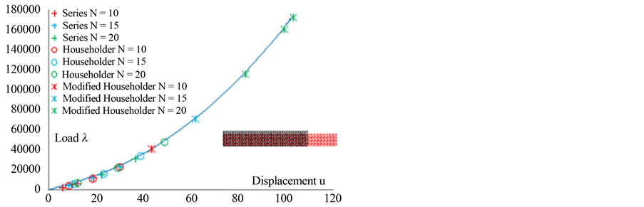
Figure 6. Traction of an elastic plate, load-displacement curve,  versus displacement u at node 246 for the three types of calculation for truncation orders 10, 15 and 20.
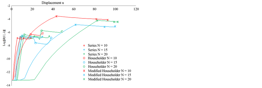
Figure 7. Traction of an elastic plate, residual curve,  as a function of the displacement u at node 246 for the three types of calculation for orders 10, 15 and 20.
fact, the orthonormalization procedure is time consuming because of the very large number of scalar products to be evaluated. It remains to explore different choices of this new class of Vector Padé approximants.
REFERENCES
- B. Cochelin, N. Damil and M. Potier-Ferry, “Méthode Asymptotique Numerique,” Hermes Science, Paris, 2007.
- B. Cochelin, N. Damil and M. Potier-Ferry, “Asymptotic Numerical Method and Padé Approximants for Nonlinear Elastic Structures,” International Journal for Numerical Methods in Engineering, Vol. 37, 1994, pp. 1187-1213. http://dx.doi.org/10.1002/nme.1620370706
- J. Van Iseghem, “Vector Padé Approximants, in Numerical Mathematics and Applications,” North Holland, Amsterdam, 1985, pp. 73-77.
- C. Brezinski, “Comparisons between Vector and Matrix Padé Approximants,” Journal of Nonlinear Mathematical Physics, Vol. 10, Suppl. 2, 2003, pp. 1-12. http://dx.doi.org/10.2991/jnmp.2003.10.s2.1
- H. Padé, “Sur la Représentation Approchée D’une Fonction par des Fractions Rationnelles,” Annales de l’Ecole Normale Supérieur, Vol. 9, 1892, pp. 3-93.
- M. Van-Dyke, “Computed-Extended Series,” Annual Review in Fluid Mechanics, Vol. 16, 1984, pp. 287-309. http://dx.doi.org/10.1146/annurev.fluid.16.1.287
- C. Brezinski and V. Iseghem, “Padé Approximants,” In: P.G. Ciarlet and J. L. Lions, Eds., Handbook of Numerical Analysis, Vol. 3, North-Holland, Amsterdam, 1994.
- G. A. Backer Jr. and P. Graves Morris, “Padé Approximants,” Encyclopedia of Mathematics and Its Application, Vol. 2, Cambridge University Press, Cambridge, 1996.
- H. De Boer and F. Van Keulen, “Padé Approximants Applied to a Non-Linear Finite Element Solution Strategy,” Communications in Numerical Methods in Engineering, Vol. 13, No. 7, 1997, pp. 593-602. http://dx.doi.org/10.1002/(SICI)1099-0887(199707)13:7<593::AID-CNM104>3.0.CO;2-V
- A. El Hage-Hussein, M. Potier-Ferry and N. Damil, “A Numerical Continuation Method Based on Padé Approximants,” International Journal of Solids and Structures, Vol. 37, No. 46-47, 2000, pp. 6981-7001. http://dx.doi.org/10.1016/S0020-7683(99)00323-6
- J. L. Batoz and G. Dhatt, “Modélisation des Structures par Elément Finis,” Edition Hermès, Paris, Vol. 1, 1990.
Appendix 1: Equations Satisfied by the Matrices  and Vectors
To determine the equations satisfied by the matrices ,
,  , and vectors
![]() we start from the truncated series of order
we start from the truncated series of order  of the vector function
 (14)
(14)
Injecting (6) and (14) into (7) yields:
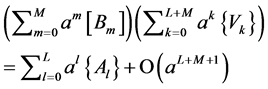 (15)
(15)
which can be written as:
 (16)
(16)
where
 (17)
(17)
 (18)
(18)
By identifying the terms corresponding to coefficients ![]() (16) we get the first
(16) we get the first  equations verified by the terms Bk :
 (19)
(19)
and that the last L equations are
 (20)
(20)
As , the matrices
 ,
,  should verify, as in the scalar case, the following system of equations:
 21)
21)
which are written in matrix form
 (22)
(22)
where:
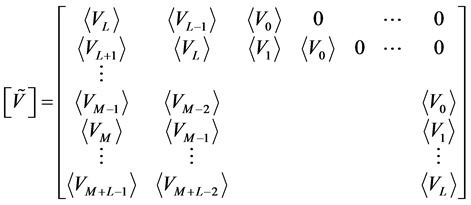 (23)
(23)
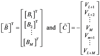 (24)
(24)
Appendix 2: Construction of Some Vector Padé Approximant
A2.1: A First Vector Padé Approximant Used in the ANM Algorithm
We will look in this part to particular solutions ,
,  , of the system (10) or (22) in the form of diagonal matrices:
 (25)
(25)
where  are the diagonal components of
  matrices.
If, for any j,  , we denote by
  the components of the vector
 , then the components of the vector
  are
are
 . Therefore if we replace in the system (8) or (16), each vector
 ,
, ,
, ![]() , by its components, we deduce, for each i,
, by its components, we deduce, for each i,  , that
  satisfy a system of the same form.
If the system has a solution, then by (9), the![]() , component of the vector
, component of the vector , is given by:
 (26)
(26)
As the matrix  is diagonal and its diagonal elements are given by
 ,
, ![]() , we conclude from (4) that the component of the Vector Padé approximant
, we conclude from (4) that the component of the Vector Padé approximant  is given by the formula (11).
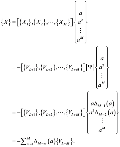
A2.2: A Second Vector Padé Approximant Used in the ANM
With the aim of building a Vector Padé approximant such that all its components are rational fractions with the same denominator, we denote by  a vector of
  of the form:
 (27)
(27)
where ,
,  are arbitrary scalars given in
  and
and  are vectors built from an orthonormalization procedure of the vectors
  such as
 (28)
(28)
Using this vector  (27), we look for the matrices
 ,
,  in the form
  where the vectors
 , are determined in order to satisfy the system (8). By replacing, in the system (8), the matrix
  by
by  and letting
  we obtain by using (28), the following equations:
 (29)
(29)
These Equation (29) show that the vectors ,
, are given by:
 (30)
(30)
Using Equation (9), we deduce that
 (31)
(31)
It is obvious that if the matrix
 (32)
(32)
is invertible, then its inverse is of the form
 where
where  is a real number. If this is the case, x satisfies
 (33)
(33)
Which is equivalent to
 (34)
(34)
As a result,
 (35)
(35)
By choosing  and posing
 (36)
(36)
equality (4) is written
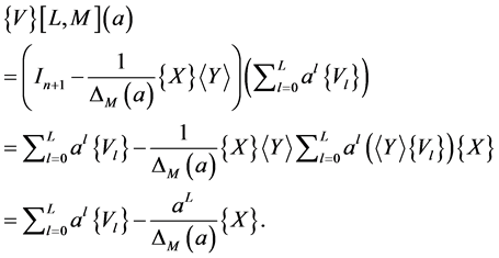
(37)
To express the Vector Padé approximant  as a function of the vectors
  , we see that if we set

and 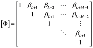 (38)
(38)
then, taking into account the equality (29), we obtain
 (39)
(39)
Hence . As Equation (29) is equivalent to
 (40)
(40)
it is concluded that:
 (41)
(41)
Using this Equation (41) in the expression of the Vector Padé approximant  (37), we find the Equation (12) which generalizes the formula of Vector Padé approximant.
A2.3: Generalization of (12)
We show in this section that in the definition of the Vector Padé approximant (37), the scalar  can be chosen arbitrarily in
 . More precisely, for
  arbitrary but fixed, there are real numbers
  such that the vector
  defined in (27) satisfies the equalities (36). Indeed, for
 , we have

Therefore, it suffices to take , so that equality (36) is satisfied. In general, for any
![]() , we have:
, we have:
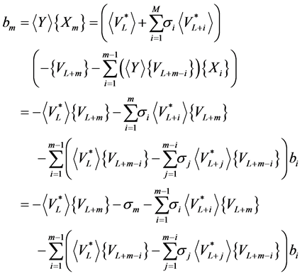
Hence, if one chooses

then we have the equality (12) for all m . Note also that if , we find the Equation (13).