World Journal of Mechanics
Vol.2 No.3(2012), Article ID:19985,5 pages DOI:10.4236/wjm.2012.23016
Application of He’s Variational Iterative Method for Solving Thin Film Flow Problem Arising in Non-Newtonian Fluid Mechanics
1Department of Mathematics, York Campus, Pennsylvania State University, University Park, USA
2COMSATS Institute of Information Technology, Abbottabad, Pakistan
3Department of Basic Sciences, Sector I-14, Riphah International University, Islamabad, Pakistan
4Department of Mathematics, COMSATS Institute of Information Technology, Islamabad, Pakistan
Email: {ams5, bsb2}@psu.edu, {aliahmedfarooq, tahirapak}@yahoo.com, mafzalrana@gmail.com
Received March 26, 2012; revised April 26, 2012; accepted May 6, 2012
Keywords: Thin Film Flow; Third Grade Fluid; Nonlinear Boundary Value Problem; Variational Iteration Method; Adomian Decomposition Method
ABSTRACT
In this paper, He’s variational iteration method is successfully employed to solve a nonlinear boundary value problem arising in the study of thin film flow of a third grade fluid down an inclined plane. For comparison, the same problem is solved by the Adomian decomposition method. The results show that the difference between the two solutions is negligible. The conclusion is that this technique may be considered an alternative and efficient method for finding approximate solutions of both linear and nonlinear boundary value problems. Furthermore, the variational iteration method has an advantage over the decomposition method in that it solves the nonlinear problems without using the Adomian polynomials.
1. Introduction
Recently, many approximate analytical and numerical methods have been suggested for solving linear and nonlinear boundary value problems arising in different branches of science and engineering. It is not difficult to solve a linear problem because of the availability of high performance digital computers, but finding solutions of nonlinear problems is still not easy. It is well known that getting an exact analytic solution of a given nonlinear problem is often more difficult compared to getting a numerical solution, despite the availability of supercomputers and software packages such as Maple, Mathe matica, Matlab etc, which provide an easy way to perform high quality symbolic computations. However, results obtained by numerical methods may give discon tinuous points of a curve when plotted; besides that complete physical understanding of a nonlinear problem is also difficult. If a nonlinear problem contains some sort of singularity or has multiple solutions then this also adds to the numerical difficulties. Though numerical and analytical solution methods have their limitations, at the same time they have their own advantages too. Therefore, we cannot neglect either of the two approaches but usually it is pleasing to solve a nonlinear problem analytically. In the recent decades, many different analytic methods have been introduced to solve the nonlinear problems, such as the homotopy analysis method (HAM) [1], the homotopy perturbation method (HPM) [2,3], the variational iteration method (VIM) [4,5], the Adomian decomposition method (ADM) [6,7], optimal homotopy asymptotic method (OHAM) [8,9]. In this study, we have applied the VIM and the ADM to find the approximate solutions of nonlinear and inhomogeneous differential equation governing the thin film flow of a third grade fluid down an inclined plane, and have made a graphical comparison of the numerical results from these two methods. Very recently, Mustafa Inc and Ebru Cavlak [10] have provided a comparative study of ADM and VIM in solving a new coupled MKdV system of equations. These methods generate the solution in a convergent series with components that are elegantly computed. Furthermore, these analytic methods avoid the complexities provided by other pure numerical methods [11,12]. The results reveal that the proposed methods provide an effective mathematical tool to handle a large class of linear and nonlinear differential equations.
2. Governing Equation
The thin film flow of a third grade fluid down an inclined plane of inclination  is governed by the following nonlinear boundary value problem [13]
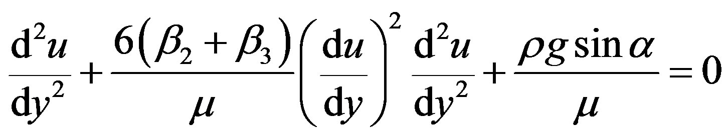 (2.1)
(2.1)
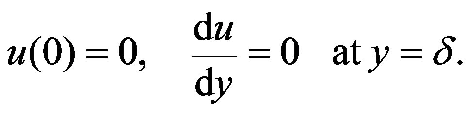 (2.2)
(2.2)
Introducing the parameters
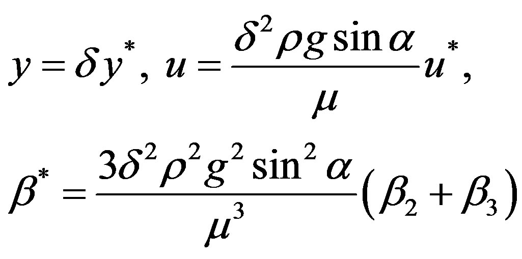 (2.3)
(2.3)
the problem in Equations (2.1) and (2.2), after omitting asterisks, takes the following form
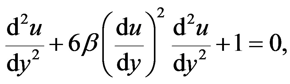 (2.4)
(2.4)
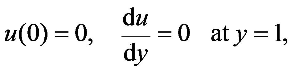 (2.5)
(2.5)
where  is the dynamic viscosity, g is the gravity,
  is the fluid density and β > 0 is the material constant of a third grade fluid. We note that Equation (2.4) is a second order nonlinear and inhomogeneous differential equation with two boundary conditions; therefore, it is a well-posed problem.
Through integration of Equation (2.4) we have
 (2.6)
(2.6)
where  is a constant of integration. Employing the second condition of (2.5) in Equation (2.6), we obtain
  = 1. Thus, the system (2.4)-(2.5) can be written as
 (2.7)
(2.7)
 (2.8)
(2.8)
It should be noted that for , Equation (2.4) corresponds to that of Newtonian fluid whose exact solution subjected to the boundary conditions (2.5) is given by
 (2.9)
(2.9)
In what follows, we will obtain the approximate analytic solutions of the nonlinear system (2.7)-(2.8) by using the VIM and the ADM techniques.
3. Solution by Variational Iteration Method
To illustrate the basic idea of He’s VIM, we consider the following nonlinear functional equation [4,5]
 (3.1)
(3.1)
where  is a linear operator,
  a nonlinear operator and
  an inhomogeneous term. Ji-Huan He has modified the general Lagrange multiplier method into an iteration method, which is called correction functional, in the following way [10]
 (3.2)
(3.2)
where  is a Lagrange multiplier that can be identified optimally via the variational theory [10]. The subscript
  denotes the
  approximation and
  is considered to be restricted variation, that is,
  The solution of the linear problem can be achieved in a single iteration step due to the exact identification of the Lagrange multiplier. This method requires the Lagrange multiplier
  be first determined optimally. The successive approximations
 of the solution
  can be readily obtained by using this determined Lagrange multiplier and any selective function
  Consequently, the solution is given by s. For the convergence criteria and error estimates of the VIM we refer the reader to [12,14].
According to the VIM, we can construct a correction functional of Equation (2.7) as follows
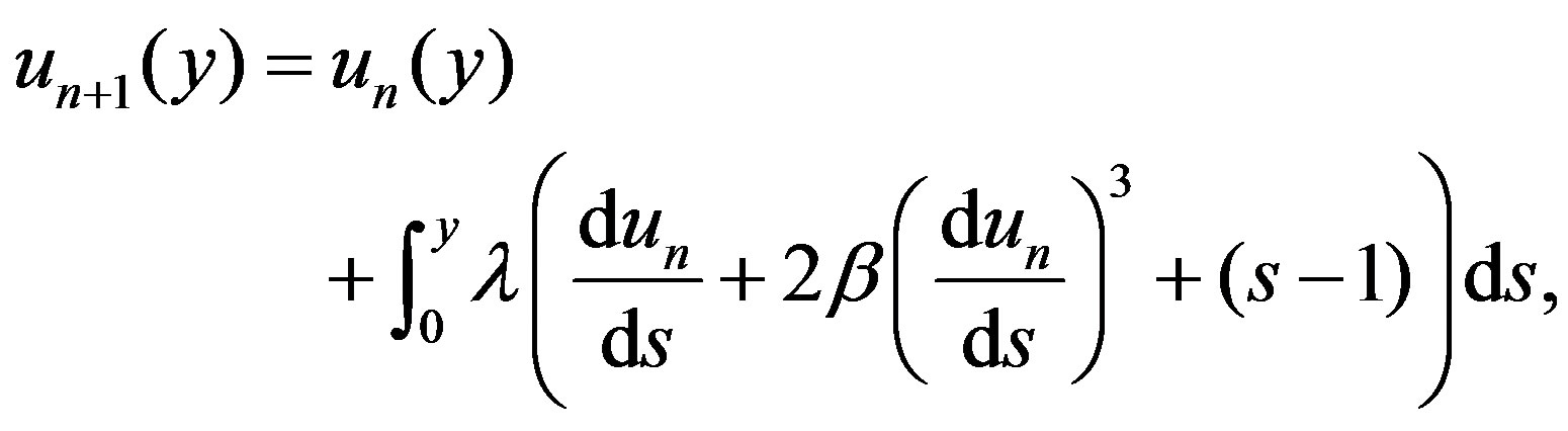 (3.3)
(3.3)
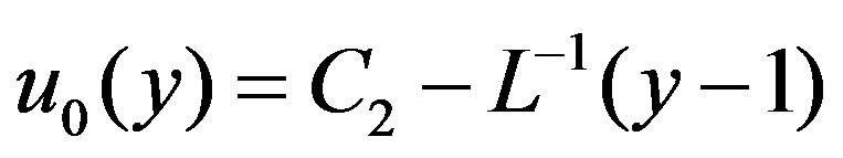
with  We start with the initial guess
  in the above iteration formula and obtain the following approximate solutions:
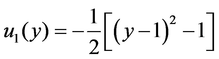 (3.4)
(3.4)
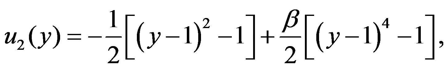 (3.5)
(3.5)
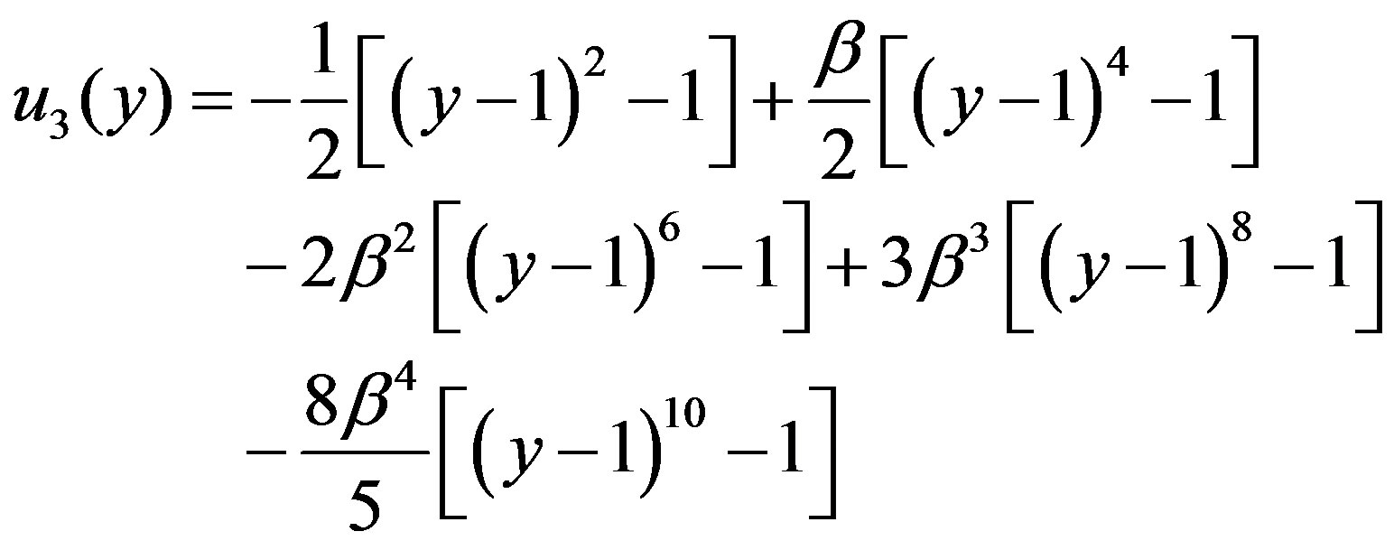 (3.6)
(3.6)
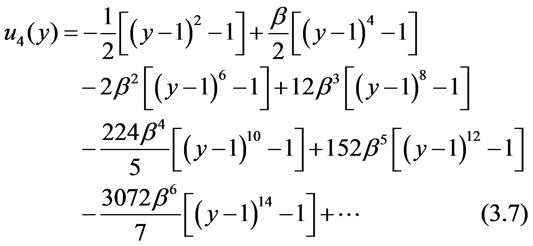

In the solution (3.7) the terms involving the powers of  gives the contribution of the non-Newtonian fluid. It is worth noting that by setting
  in the above approximations, we recover the exact solution for the case of Newtonian fluid. Thus, the first approximation of the nonlinear system (2.7)-(2.8) obtained by the VIM is identical with the exact solution of the corresponding linear problem. This shows that the VIM can be equally applied to linear equations.
The effects of the non-Newtonian parameter  on the velocity given in (3.7) are plotted in Figure 1. It is shown that as we decrease the non-Newtonian parameter
  the solution converges to the Newtonian case.
4. Solution by Adomian Decomposition Method
A detailed description of the ADM is given in [6,7]. Here, we convey only the basic steps as a reminder. Writing Equation (2.7) in operator form, we obtain
 (4.1)
(4.1)
where 
 ,
, .
.
Here,  is the highest order derivative which is assumed to be easily invertible,
  represents the nonlinear term and
  is the source term. According to the ADM, the solution
  can be expanded into the infinite series
 (4.2)
(4.2)
where the components  are usually determined recursively. The nonlinear term
  can be decomposed into infinite polynomials given by
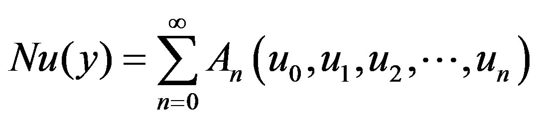 (4.3)
(4.3)
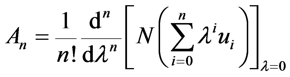
where  are the so-called Adomian polynomials of
  defined by
 (4.4)
(4.4)
or equivalently,
 (4.5)
(4.5)

It is well known that these polynomials can be constructed for all classes of nonlinearity according to the algorithm set by Adomian [15].
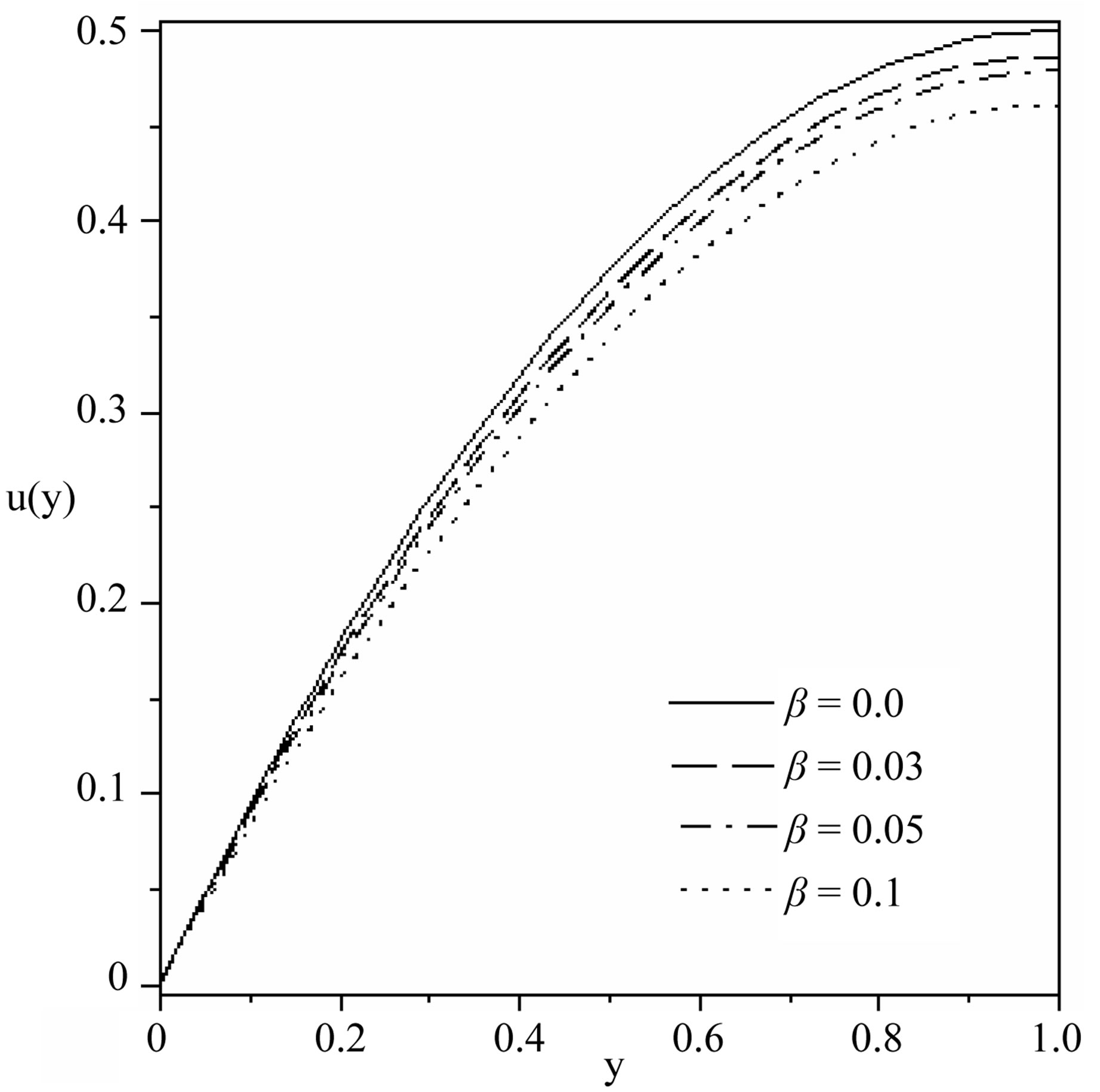
Figure 1. Variations in velocity with y for different values of β.
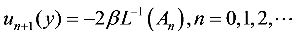
The general algorithm of this decomposition method for the nonlinear system (2.7)-(2.8) yields the recurrence relation,
 (4.6)
(4.6)
 (4.7)
(4.7)
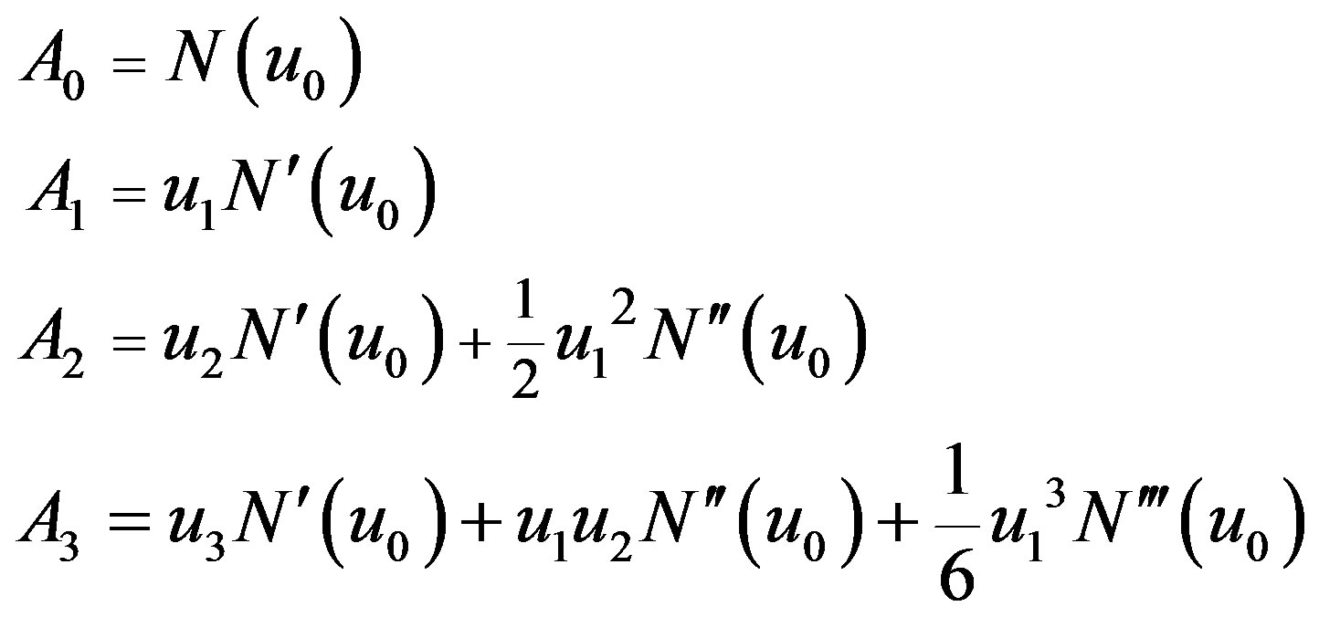
where C2 is a constant of integration and can be found from the boundary condition (2.8). The first few terms of the Adomian polynomials 
 for this problem are given by:
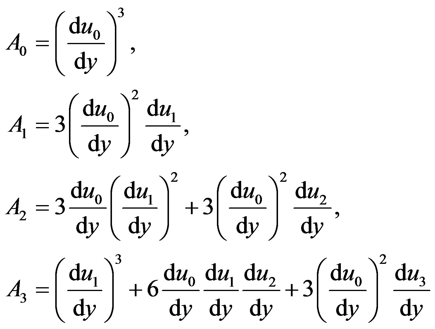 (4.8)
(4.8)

From these above results, we obtain the following components
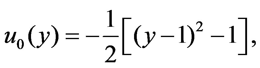 (4.9)
(4.9)
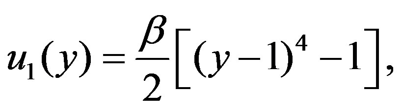 (4.10)
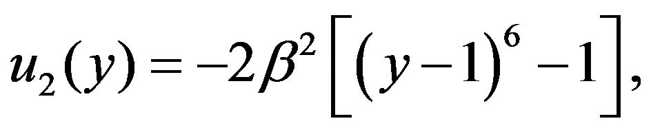 (4.11)
 (4.12)
 (4.13)
 (4.14)
In this manner, the rest of the terms in the decomposition series can be calculated. Summing up, we write the solution in the decomposition series form
This, after inserting the values of  and
and  from (4.9)-(4.14), becomes
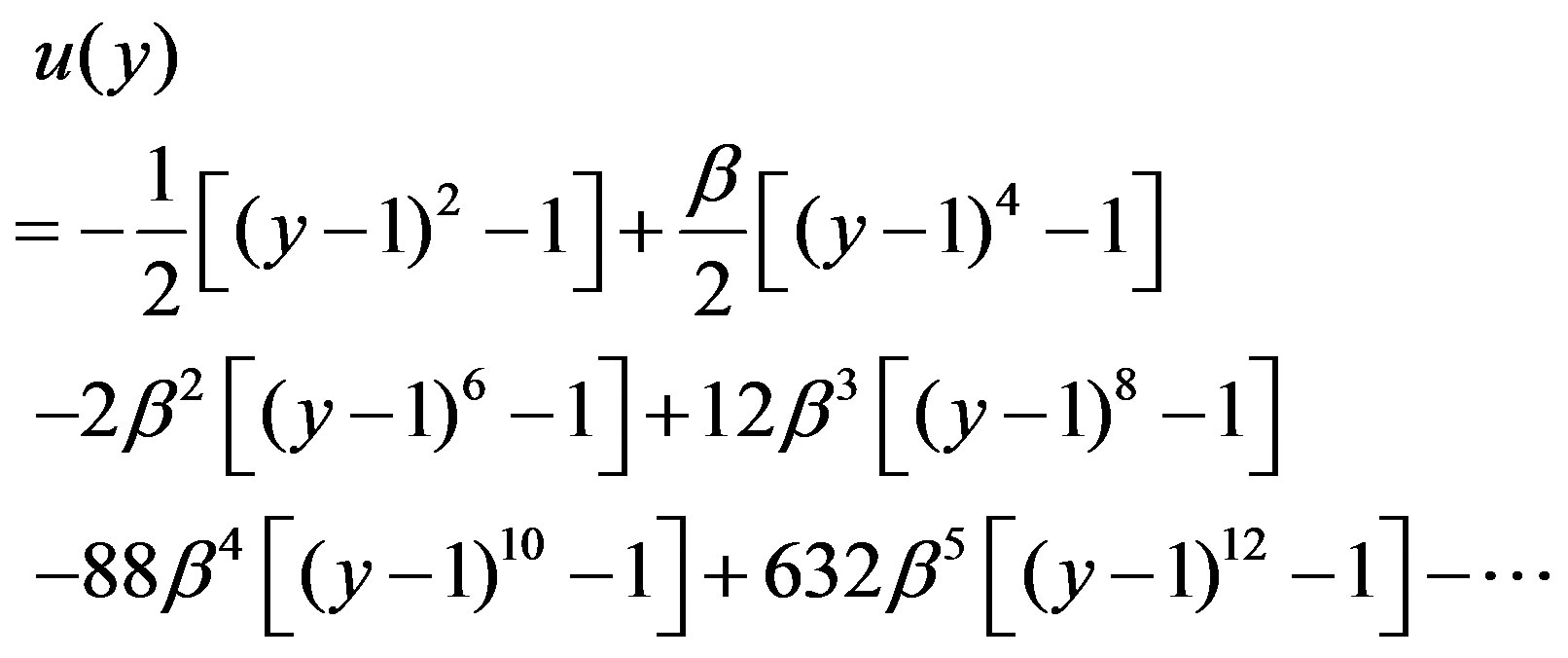 (4.15)
which is the same as that obtained by the VIM. As before, setting  in (4.15) one can recover the exact solution for the Newtonian fluid.
5. Conclusion
In this study, we have illustrated how the VIM and the ADM can be employed to obtain the approximate analytical solution of a nonlinear boundary value problem arising in the study of non-Newtonian fluid mechanics. The comparison between the fourth iteration solution of the VIM and five terms of the ADM is given in Figure 2. In fact, for  an excellent agreement is observed.
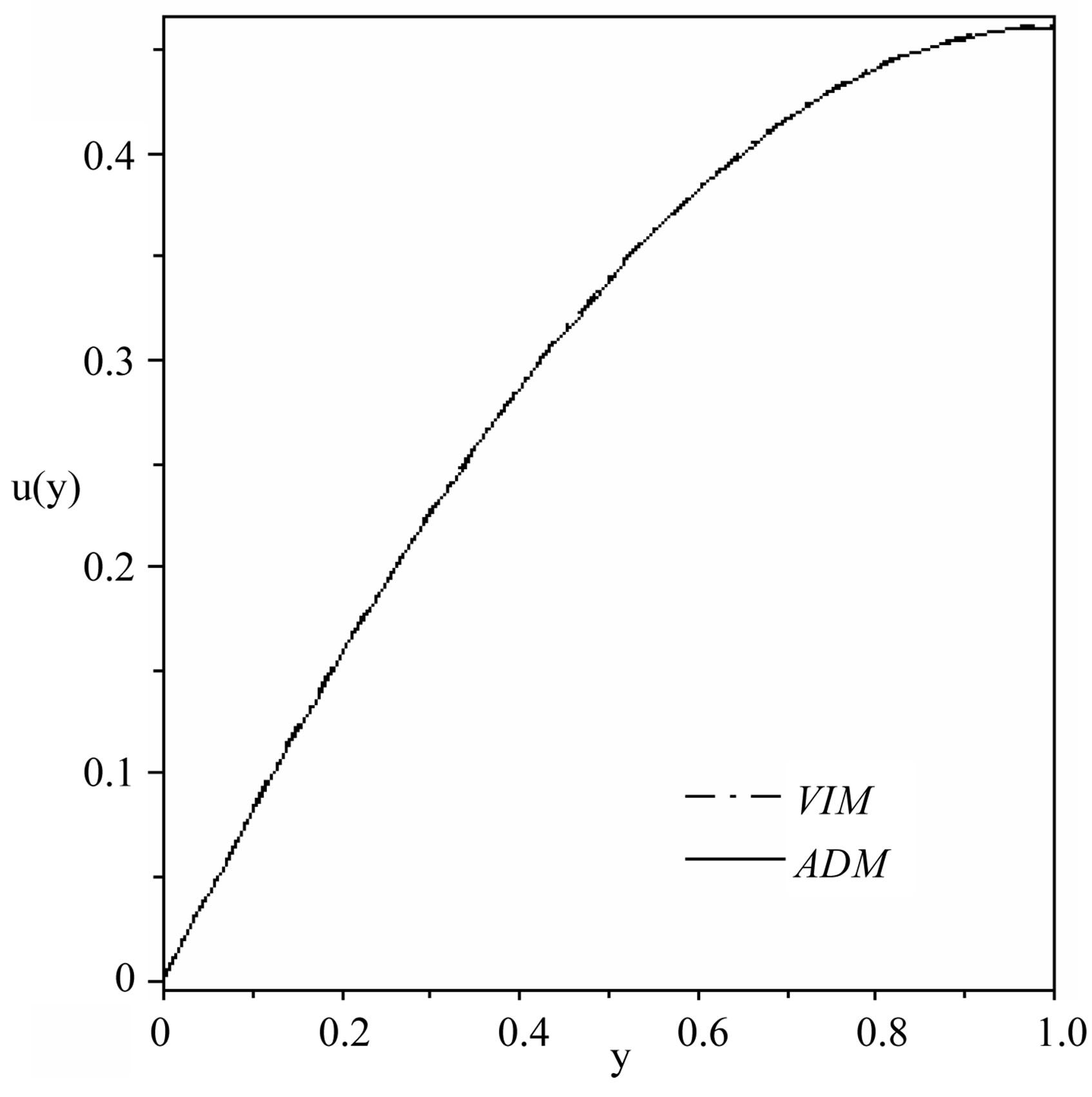
Figure 2. Comparison of the VIM solution and the ADM solution, when β = 0.05.
Therefore, these methods are very powerful and efficient techniques for solving different kinds of linear and nonlinear problems arising in various fields of science and engineering. However, the VIM has an advantage over the ADM in that it solves the nonlinear problems without using the Adomian polynomials. Also, the use of the Lagrange multiplier reduces the successive use of the integral operator and it may be considered as an added advantage of this technique over the decomposition method.
REFERENCES
- S. J. Liao, “Beyond Perturbation: Introduction to Homotopy Analysis Method,” Chapman & Hall/CRC Press, Boca Raton, 2004.
- J. H. He, “Homotopy Perturbation Technique,” Computer Methods in Applied Mechanics and Engineering, Vol. 178, No. 3-4, 1999, pp. 257-262. doi:10.1016/S0045-7825(99)00018-3
- J. H. He, “A Coupling Method of a Homotopy Technique and a Perturbation Technique for Non-Linear Problems,” International Journal of Non-Linear Mechanics, Vol. 35, No. 1, 2000, pp. 37-43.
- J. H. He, “Variational Iteration Method—A Kind of NonLinear Analytical Technique: Some Examples,” International Journal of Non-Linear Mechanics, Vol. 34, No. 4, 1999, pp. 699-708. doi:10.1016/S0020-7462(98)00048-1
- J. H. He, “Variational Iteration Method—Some Recent Results and New Interpretations,” Journal of Computational and Applied Mathematics, Vol. 207, No. 1, 2007, pp. 3-17.
- G. Adomian, “Solving Frontier Problems of Physics: The Decomposition Method,” Kluwer Academic Publishers, Boston, 1994.
- G. Adomian, “A Review of the Decomposition Method in Applied Mathematics,” Journal of Mathematical Analysis and Applications, Vol. 135, No. 2, 1988, pp. 501-544. doi:10.1016/0022-247X(88)90170-9
- V. Marinca and N. Herisanu, “Application of Optimal Homotopy Asymptotic Method for Solving Nonlinear Equations Arising in Heat Transfer,” International Communications in Heat and Mass Transfer, Vol. 35, No. 6, 2008, pp. 710-715. doi:10.1016/j.icheatmasstransfer.2008.02.010
- S. Islam, Z. Bano, I. Siddique and A. M. Siddiqui, “The Optimal Solution for the Flow of a Fourth-Grade Fluid with Partial Slip,” Journal Computers & Mathematics with Applications, Vol. 61, No. 6, 2011, pp. 1507-1516. doi:10.1016/j.camwa.2011.01.014
- M. Inc and E. Cavlak, “On Numerical Solutions of a New Coupled MKdV System by Using the Adomian Decomposition Method and He’s Variational Iteration Method,” Physica Scripta, Vol. 78, No. 4, 2008, pp. 1-7. doi:10.1088/0031-8949/78/04/045008
- N. Bildik and A. Konuralp, “Two-Dimensional Differential Transform Method, Adomian’s Decomposition Method, and Variational Iteration Method for Partial Differential Equations,” International Journal of Computer Mathematics, Vol. 83, No. 12, 2006, pp. 973-987. doi:10.1080/00207160601173407
- J. I. Ramos, “On the Variational Iteration Method and Other Iterative Techniques for Nonlinear Differential Equations,” Applied Mathematics and Computation, Vol. 199, No. 1, 2008, pp. 39-69. doi:10.1016/j.amc.2007.09.024
- A. M. Siddiqui, R. Mahmood and Q. K. Ghori, “Homotopy Perturbation Method for Thin Film Flow of a Third Grade Fluid Down an Inclined Plane,” Chaos, Solitons & Fractals, Vol. 35, No. 1, 2008, pp. 140-147. doi:10.1016/j.chaos.2006.05.026
- M. Tari and M Dehghan, “On the Convergence of He’s Variational Iteration Method,” Journal of Computational and Applied Mathematics, Vol. 207, No. 1, 2007, pp. 121-128. doi:10.1016/j.cam.2006.07.017
- A. M. Siddiqui, M. Hameed, B. M. Siddiqui and Q. K. Ghori, “Use of Adomian Decomposition Method in the Study of Parallel Plate Flow of a Third Grade Fluid,” Communication in Nonlinear Science and Numerical Simulation, Vol. 15, No. 9, pp. 2388-2399, 2010. doi:10.1016/j.cnsns.2009.05.073