World Journal of Mechanics
Vol.2 No.1(2012), Article ID:17680,10 pages DOI:10.4236/wjm.2012.21002
Numerical Investigation of Flow Structure Interaction Coupling Effects in Hard Disk Drives
1School of Mechanical & Aerospace Engineering, Nanyang Technological University, Singapore
2Data Storage Institute, Agency for Science, Technology and Research, Singapore
Email: *mykng@ntu.edu.sg
Received November 7, 2011; revised December 10, 2011; accepted December 20, 2011
Keywords: Hard Disk Drives; Coupling Method; Modeling; Simulation and Optimization; FSI
ABSTRACT
This paper studies the flow structural interaction (FSI) within a hard disk drive (HDD) through the use of a novel coupling method. The interaction studied was the fluid induced vibration in the HDD. A two step coupling approach was used, where the fluid and structural components were solved sequentially. The result obtained was a ratio of 0.65 between the vibration amplitudes of a fixed head stack assembly (HSA) and a moving HSA. The ratio was next applied on a real 3.5 inch HDD, to allow the parameter to be further improved upon. A new benchmark index of 0.69 was developed from this. This parameter may allow future researchers to model the out of plane vibrations of a HSA easily, saving precious time. A 31% more accurate simulation of FSI within 3.5 inch HDD at 15000 rpm is achieved by the use of this new coupling method and benchmark index.
1. Introduction
Fluid structure interaction (FSI) is the interaction between structures and internal or external surrounding fluid. The behavior of the structure is influenced by both the flow field of the surrounding fluid and the flow field of the structure [1]. These interactions play an important role in the design of many engineering systems. Examples include bridges, aircrafts and hard disks [1]. FSI includes the influences of both the structure and the fluid. The interaction happens at the interface between the fluid domain and the structure domain.
FSI problems are typically very complex, hence are seldom solved analytically. Numerical simulation is usually used to solve FSI problems. However, the numerical simulation of FSI problems is complicated as it possesses problems associated with both fluid and structural simulation. In addition, the coupling of the fluid and structural interface is also challenging [2].
There are two approaches that can be taken to solve FSI problems using numerical simulation, namely: the strong and the weak coupling methods. For the strong coupling method, the governing equations for the fluid and structure are solved simultaneously with a single solver. Generally, it leads to a convergence rate of the 2nd order [2,3]. However, the strong coupling method is of limited use as it requires the modification of existing fluid and structural solvers, there is restricted flexibility between the time integration and mesh discretization of the fluid and structural solvers. In addition, strong coupling also requires extensive computational power and storage requirements. While for the weak coupling method, the governing equations for the fluid and structure are solved separately with two different solvers. The results from the fluid solver and structural solver are inputted into each other sequentially and iteratively. Hence this allows existing solvers to be used easily. However, there is a greater chance of convergence problem for the weak coupling method [3].
Due to the complexity of the geometry of HDD and the fact that FSI for HDD lies the nanometer scale (& hence may consider avoid remeshing due to small deformations), the strong coupling method is inefficient for solving such problems in this paper. In addition, despite recent advancements in FSI, there are still problems associated with the accuracy of the force transfers between fluid and structural domain, and the effectiveness of weak coupling approaches [4]. The high frequency vibration of the HSA also makes strong coupling unsuitable for this scenario. Hence a modified weak coupling method where the fluid and structural components are solved sequentially is used for the purpose of this FSI study.
In addition, there is a need to develop a better method or higher order schemes like the spectral difference [5], spectral volume [6] and the continuous Galerkin [7] to solve such problems and hence lead to the development of better HDD.
2. Preliminary Studies
2.1. Numerical Solvers
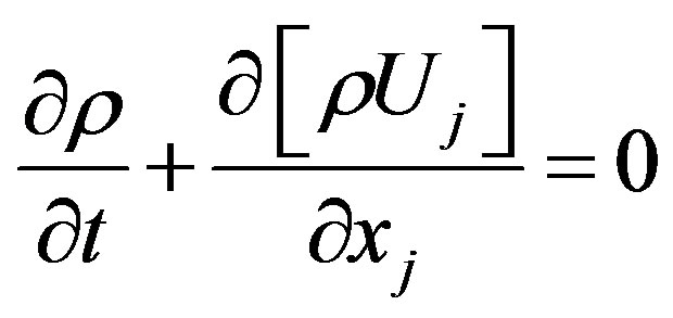
The 3 basic standard governing equations used in the Fluent are: continuity (1), momentum (2) and energy equation (3) for unsteady compressible fluid and can be written as with usual definitions:
 (1)
(1)
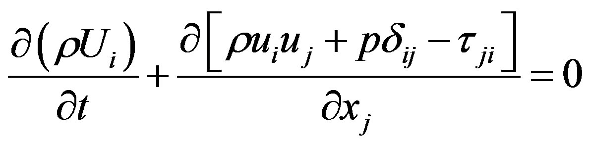 (2)
(2)
 (3)
(3)
In Equations (1) to (3), ρ is the density, p is the pressure,  is the isotropic tensor or Kronecker delta, U is the velocity vector, ui is the velocity components, x is in Cartesian space, eo is total energy per unit volume and
  the viscous stresses. The suffices i and j in
  indicate that the stress component acts in the j-direction on a surface normal to the i-direction.
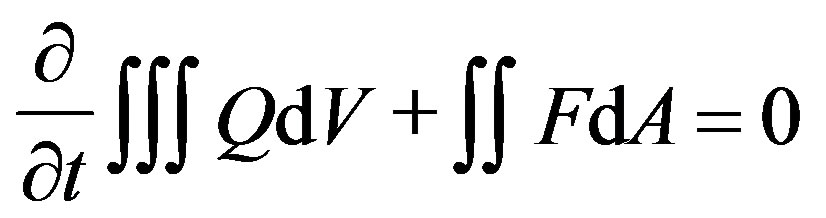
The finite volume method (FVM) is used in Fluent code. The governing equations are solved over discrete control volumes. FVMs recast the governing partial differential equations in a conservative form, and then discretize the new equation. This guarantees the conservation of fluxes through a particular control volume. The finite volume equation yields governing equations in the form,
 (4)
(4)
where Q is the vector of conserved variables, F is the vector of fluxes in Navier-Stokes equations, V is the volume of the control volume element, and A is the surface area of the control volume element.
The finite element method (FEM) is used in structural analysis of solids (ANSYS [8]), though is also applicable to fluids. However, the FEM formulation requires special care to ensure a conservative solution. The FEM formulation has been adapted for use with fluid dynamics governing equations. Although FEM must be carefully formulated to be conservative, it is much more stable than the finite volume approach. However, FEM can require more memory than FVM.
In this method, a weighted residual equation is formed:
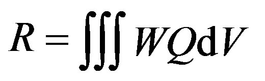 (5)
(5)
where R is the equation residual at an element vertex i, Q is the conservation equation expressed on an element basis, W is the weight factor, and V is the volume of the element.
2.2. Mesh Dependency Study
The aim of this simulation is to perform a mesh dependency study of a simplified HDD. This is achieved by creating a simplified model of a commercial HDD, and simulating the airflow patterns within it. This would allow the user to understand the mesh size required to obtain accurate results when performing further simulation for more complex cases.
The model and mesh was created using a commercial software GAMBIT. The airflow simulation was done with FLUENT, a popular software used for computational fluid dynamics (CFD).
Figure 1 shows a side view of the disk case with all relevant geometric data. The origin of coordinates is located at the center of bottom disk surface. The boundary conditions are found in Table 1. The mesh data is included in Table 2, while the computer specifications for running this simulation are given in Table 3. A total of

Figure 1. Side view of disk case (all dimensions are in mm).

Table 1. Boundary conditions applied to simplified HDD.
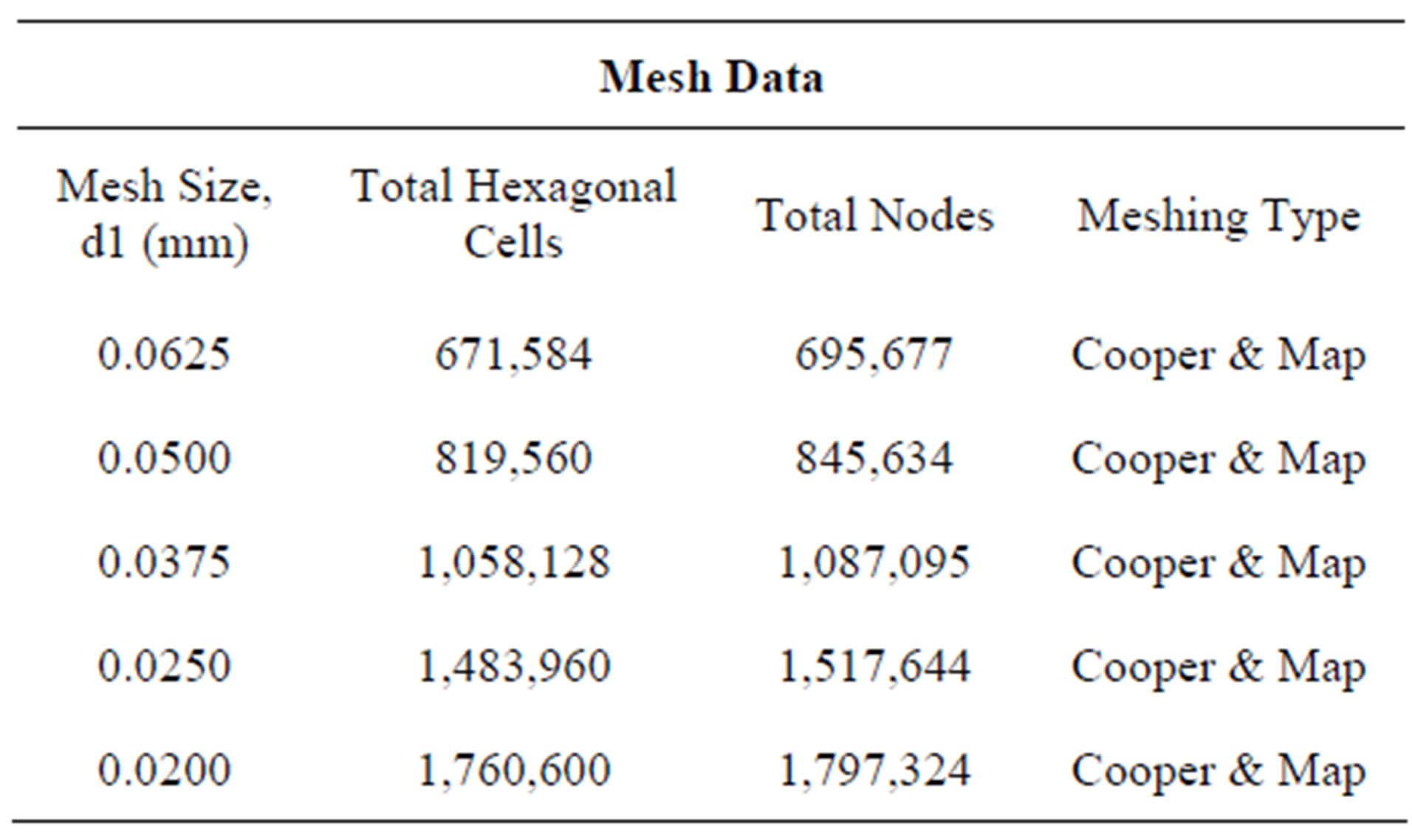
Table 2. Mesh data tested.
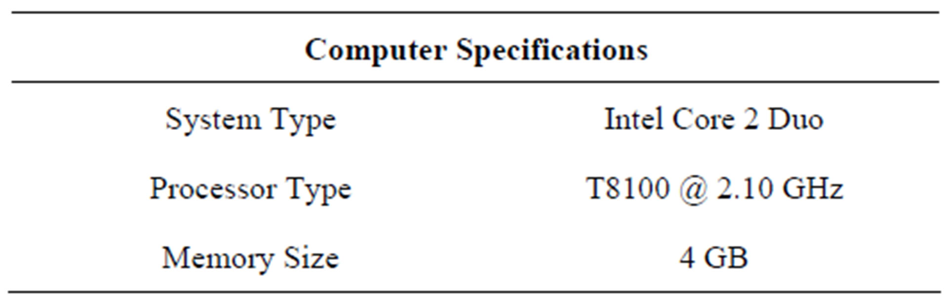
Table 3. Computer specifications.
four models were created with varying fineness in meshing. The case is solved as a 3D problem. Here, d1 is the size of the smallest mesh closest to the boundaries.
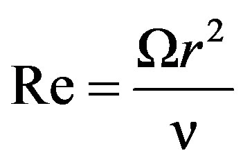
For a pair of co-rotating disks, Reynolds number is given as follows:
 (6)
(6)
where, Ω = angular velocity, r = disk radius, ν = kinematic viscosity.
For the present case setup, Ω = 15,000 rpm = 500π rad/s; r = 47.5 mm = 0.0475 m.
With ambient temperature of 298 K, and standard atmospheric conditions, ν = 15.43 × 10⁻⁶ m2/s, Re = 22.97 × 10⁴. Considering a critical Reynolds number of 2 × 10⁴ [9], the stated case setup has turbulent flow. Fluent’s K-ε model was used, and the transient simulations were run for 300 iterations.
Figure 2 presents the graph of pressure against the size of the smallest mesh closest to the disk for the sampling position of x = 47 mm, z = 0.8 mm, y = 0 mm. It can be observed that as the mesh gets refined, the pressure at that position drops.
Table 4 indicates that, the pressure difference between the finest and coarsest mesh can be as great as 43.1%. This represents that if the mesh is not sufficiently fine, there could be an error of 43.1% in the results. When the mesh is refined from 0.025 mm to 0.020 mm, there is very little difference pressure difference of 0.0116%. This suggests that there is no need to further refine the mesh from 0.025 mm. This grid size may be used as base-line reference when creating the mesh for the FSI study of a 3.5 inch HDD.
2.3. Fluid Structure Interaction Study of Simplified HDD
We involve here the use of the weak coupling method to investigate the FSI between the air flow around a HSA and the vibrations of the HSA for a simplified HDD case. During the normal operation of a HDD, the hard disk plates are constantly spun by a motor, inducing turbulent flow for the air around the plates. The fluid flow will in
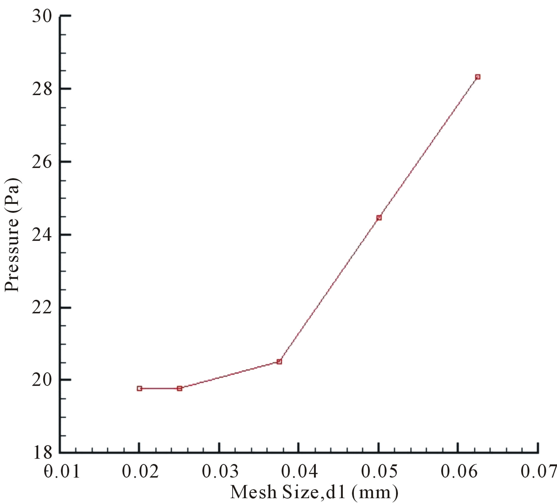
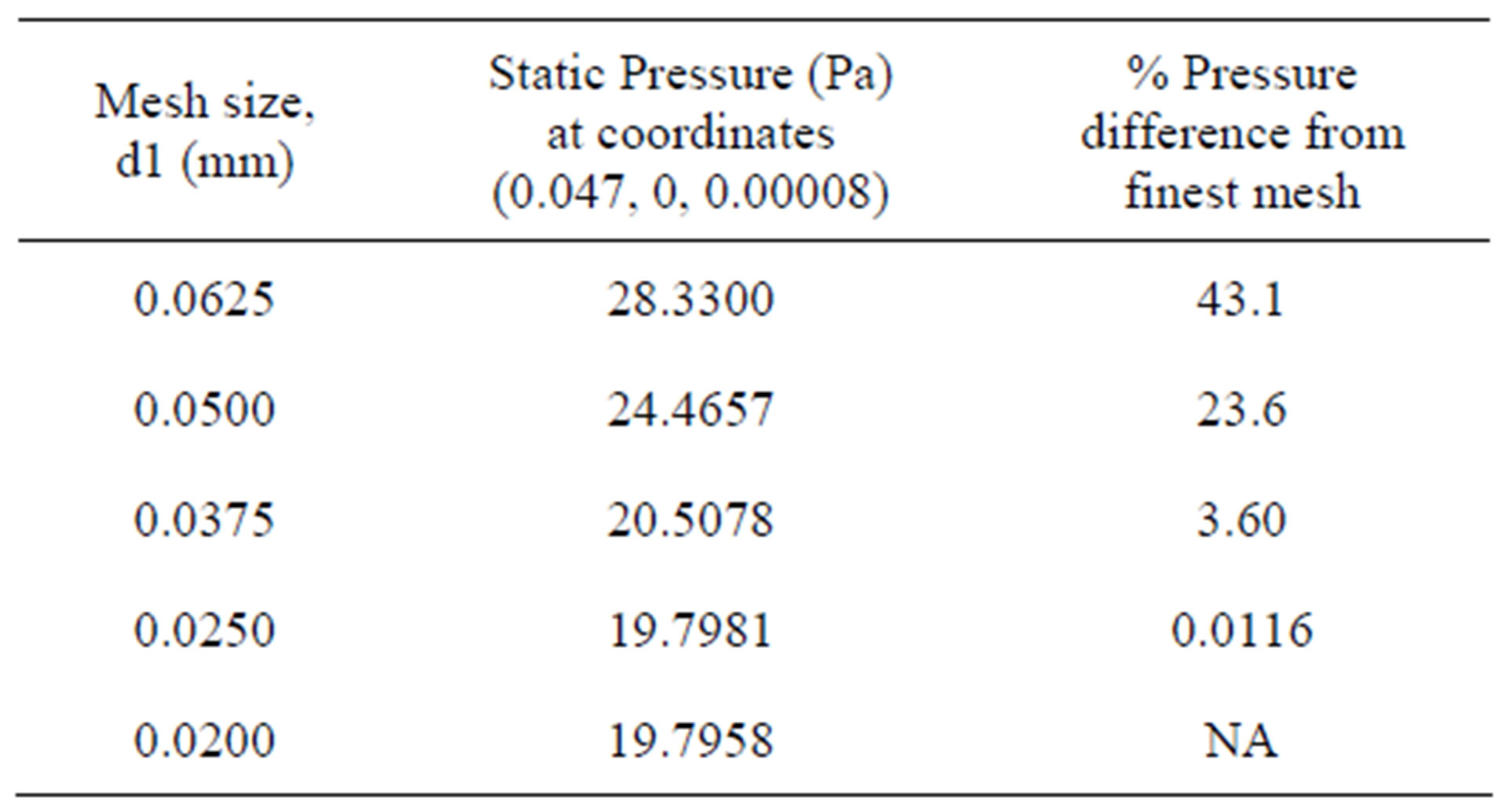
Table 4. Study of % pressure difference vs. refinement of mesh size.
turn cause the HSA to vibrate at very high frequencies of 1200 Hz [10], and these vibrations will affect the fluid flow. The complexity of this FSI within the HDD means that a large amount of computation time would be required if strong coupling is used and hence the choice of weak coupling. In-house Fortran code (InputGen) would be used to transfer the forces from CFD FLUENT to Structure ANSYS. The solving methodology of FSI is:
1) Solve the fluid components using FLUENT.
2) Transfer forces on all nodes on HSA over to the structural model.
3) Solve the structural components with ANSYS.
4) Transfer the ANSYS results to FLUENT by simulating vibrations of HSA, and repeat from step 1 until convergence is achieved.
5) Upon convergence, the ratio of the converged amplitude against the initial amplitude would be applied on a 3.5 inch hard disk to obtain a benchmark parameter.
2.3.1. Case Setup for Fluid Component
Figure 3 presents the side view of the disk case and HSA with all relevant geometric data. The coordinates system is the same as that in Figure 1. The mesh type used is “Cooper & Map” with 2722888 hexagonal cells and 2883985 nodes. The computer specifications for running this simulation are 2 × Quad-Core Nehalem x5570, 2.93 GHz processor and 16 GB memory.
With Reynolds number of Re = 22.97 × 10⁴, the case was setup to run RNG k-ε (1000 iterations) followed by LES (10000 time steps, step size = 2 × 10⁻⁶ & 5 iterations per step) simulation as tabulated in Table 5.
2.3.2. Structural Analysis Using ANSYS
The forces on the HSA due to the rotation of the disk were extracted and exported from Fluent. The case setup for the force exporting is 20000 time steps with 10 revolutions (2 steps for every force data). Due to the HSA’s relatively small vibration magnitudes in both the X and Y directions as compared to the Z direction [10], the vibrations in the X and Y directions would not be considered. They are however still considered during the structural analysis, but not be inputted into Fluent and the HSA is assumed to vibrate in the Z direction only during the next LES simulation. The material of the HDD is stainless steel. The disk revolved 5 turns during the LES simulation and 10 turns during the force extraction.
The numerical steps include:
1) Model of HSA was created using Pro-E, a commercial CAD software.
2) Mesh of HSA was created using ANSYS 12 based on the Pro-E model.
3) Boundary conditions and material properties associated to the mesh used were adjusted to ensure that the natural frequencies match results obtained from the previous experiments.
4) An in-house developed Fortran code was used to generate the required ANSYS input file and interpolating the forces exported from Fluent (Section 2.4.2) onto the mesh in ANSYS.
5) ANSYS transient analysis was ran to obtain the x, y and z direction displacements of the HSA.
6) The displacements are modeled as a cosine function and velocity of the vibrations can be modeled as a sine

Figure 3. Side view of disk case and arm (all dimensions are in mm).
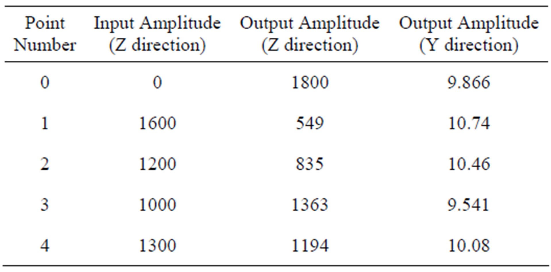
Table 5. Input amplitude vs. output amplitude for LES simulation.
function [11].
7) The frequency of the sine function was obtained through Fast Fourier Transform (FFT) of the ANSYS results. While amplitude was determined by observing the average and standard deviations of the ANSYS results.
8) The end results are inputted into Fluent through the use of a User Defined Function to carry on with the FSI analysis.
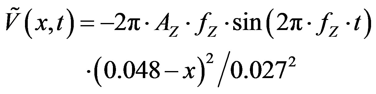
Figure 4 shows the structural model of the HSA used for this study. The HSA’s displacement in the Z direction against time is included in Figure 5. It is obvious that the HSA vibrates in a cyclic manner that could be modeled as a cosine function. Hence FFT was performed on the data and the 1st highest peak (or 1st bending) would indicate the frequency to be used in modeling the vibrations as a cosine function. Figure 6 suggests the frequency of the highest peak can be read off as 1125 Hz. The amplitude for the cosine function was 1800nm by observing the average amplitude and standard deviation of different sections (Figure 7). However, as there is currently no standard method for choosing the input amplitude, a value of 1600 was selected to be the first input. 1600 represents smaller amplitude then the observed 1800, and is thought to be helpful in achieving convergence faster for future iterations. Now, we are able to obtain the cosine function that represents the vibrations in the Z direction. By performing differentiation, the velocity function that controls the HSA’s vibrations can then be obtained as [10]:
 (7)
(7)
where,  is amplitude,
  is frequency, t is time,
  is the node position along x direction.
This amplitude of the arm is made to vary in the x direction by the 2nd order, where the displacement at the root would be the smallest, while the displacement at the end is the greatest.
2.3.3. Further LES Simulation
For subsequent simulations, the vibration of the HSA is
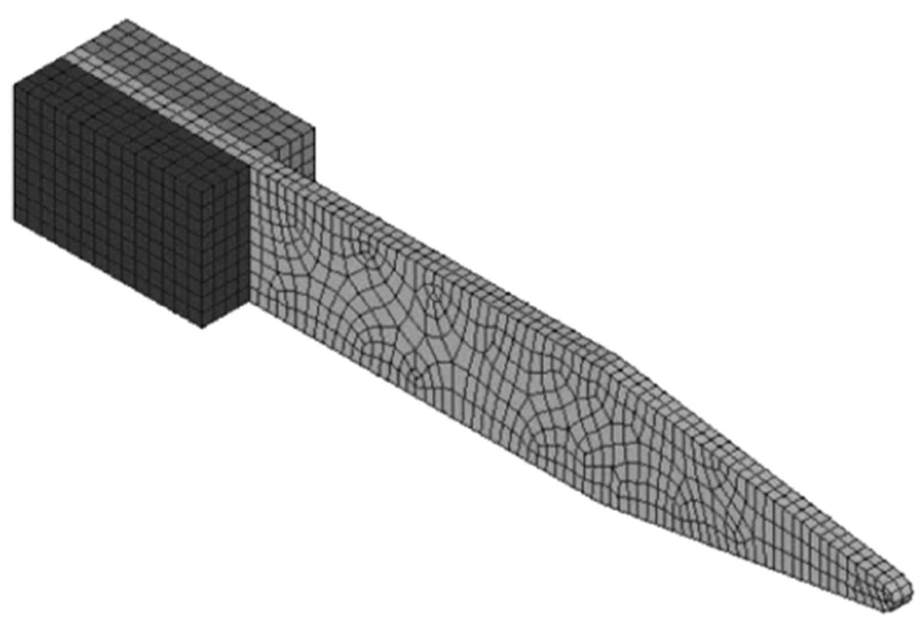
Figure 4. Structural model of HSA (isometric view).
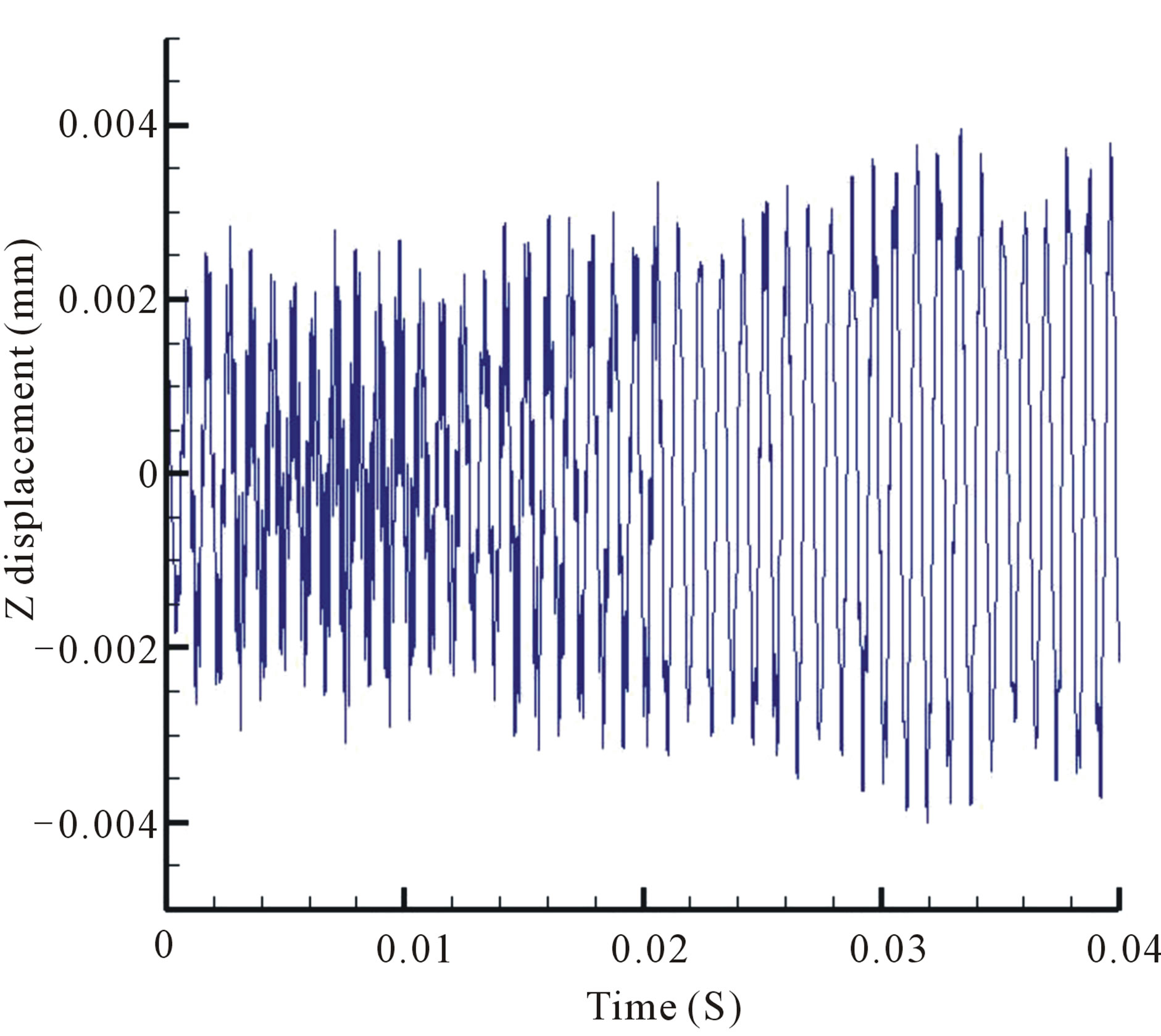
Figure 5. HSA’s Z-displacement vs. time for structural analysis.
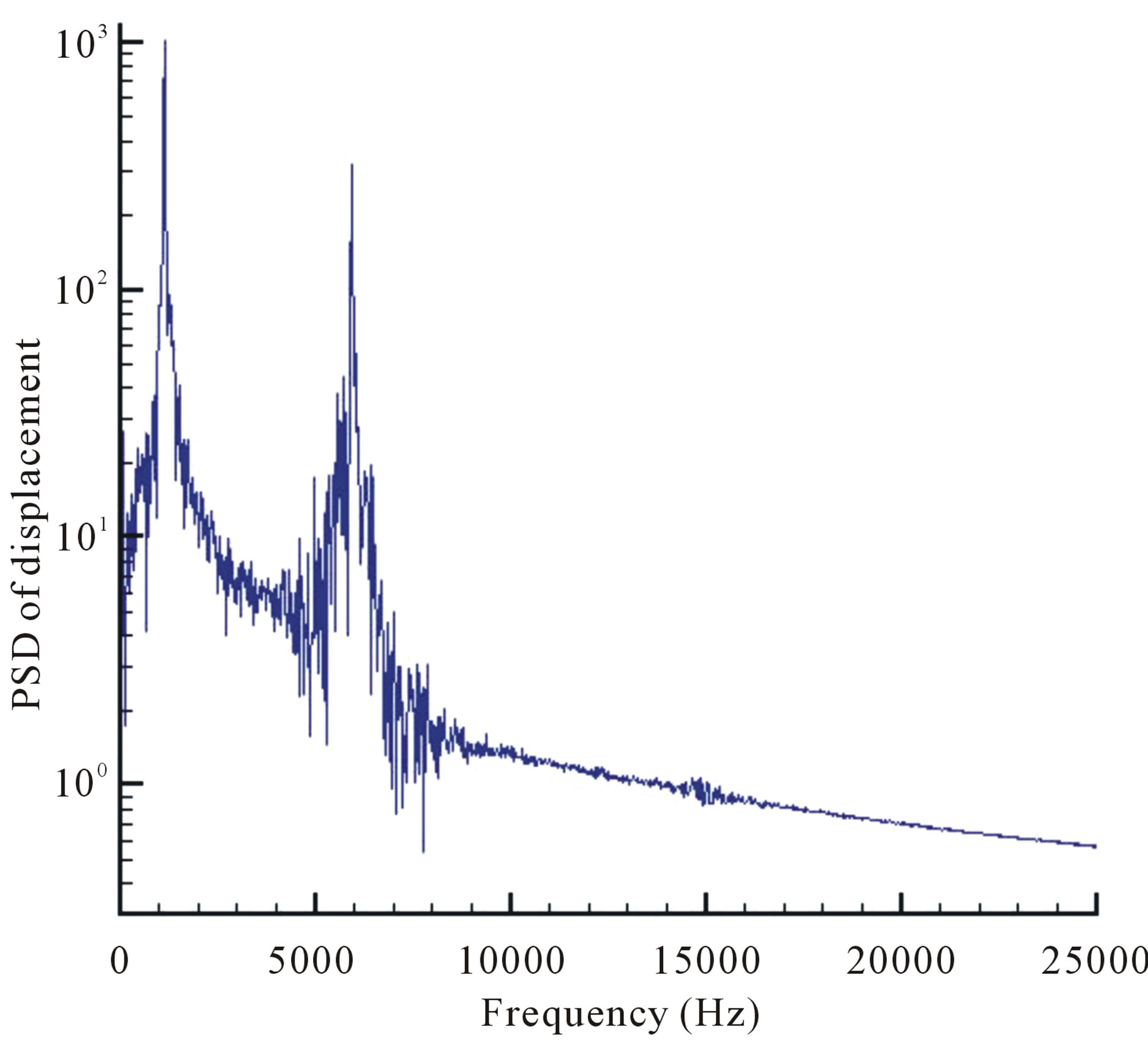
Figure 6. HSA’s displacement in Z-direction vs. frequency.
inputted into Fluent through a user defined function (UDF). The case set up is identical to the previous 1st simulation, except for the additional UDF which simulates the vibration of the HSA in the Z direction.
Figure 8 shows the convergence sequences of the FSI simulations in the Z direction (out of plane), and Y direction (off track) respectively. Complete convergence is achieved when the point lies on the “output = input” line. However, as the geometry in our case is relatively complex, with turbulent flow, complete convergence is impossible to achieve. Figure 7 shows that point 4 lies close to the “output = input” line with the difference between input and output amplitude of |input – output|/output = 0.08 which is close enough to assume a good convergence.
Figure 8 shows that the output amplitude in the Y direction does not differ much. The average of the 5 points is 10.14, and the difference between the highest and average point is just 5.9%.
Figure 9 presents the comparison plot of Y axis vs. out of plane velocity at location of Z = 9.725 mm and X = 34 mm. This plot compares the out of plane velocity of the fixed HSA and moving (vibrating) HSA case. Fixed HSA refers to point 0, where the input amplitude is 0 nm, and the HSA is assumed to be fixed. Moving HSA refers to point 4 where the input amplitude is 1300 nm. It is obvious that the fixed HSA case has a significantly higher velocity as compared to the moving HSA case since the fixed HSA is blocking the surrounding air flow and hence resulting in strong vibrations. The moving HSA is however modeled to vibrate, it would “block” the surrounding air flow to a less extent and thus giving a lower out of plane velocity.
The FSI study reveals the ratio of the converged am

Figure 7. HSA’s output amplitude vs. input amplitude (Z direction).
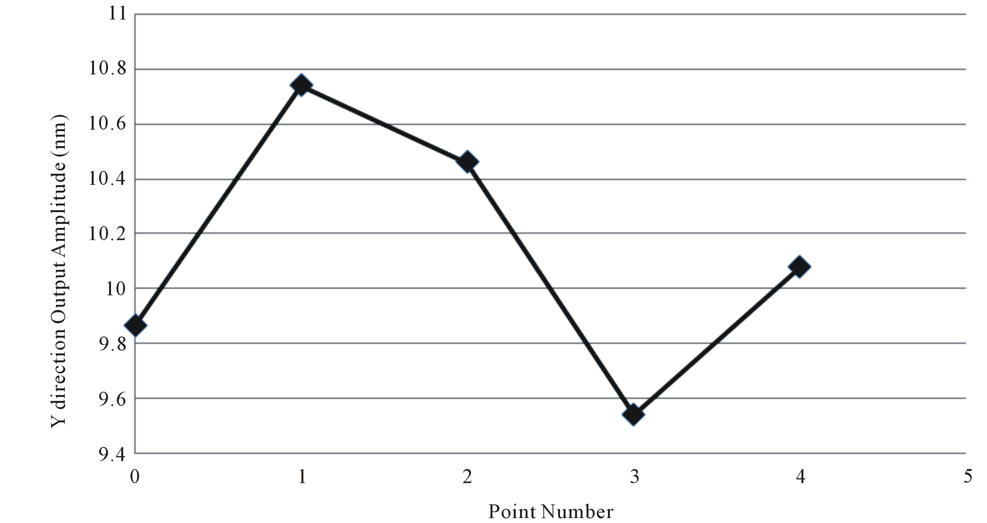
Figure 8.HSA’s output amplitude vs. point number (Y direction).

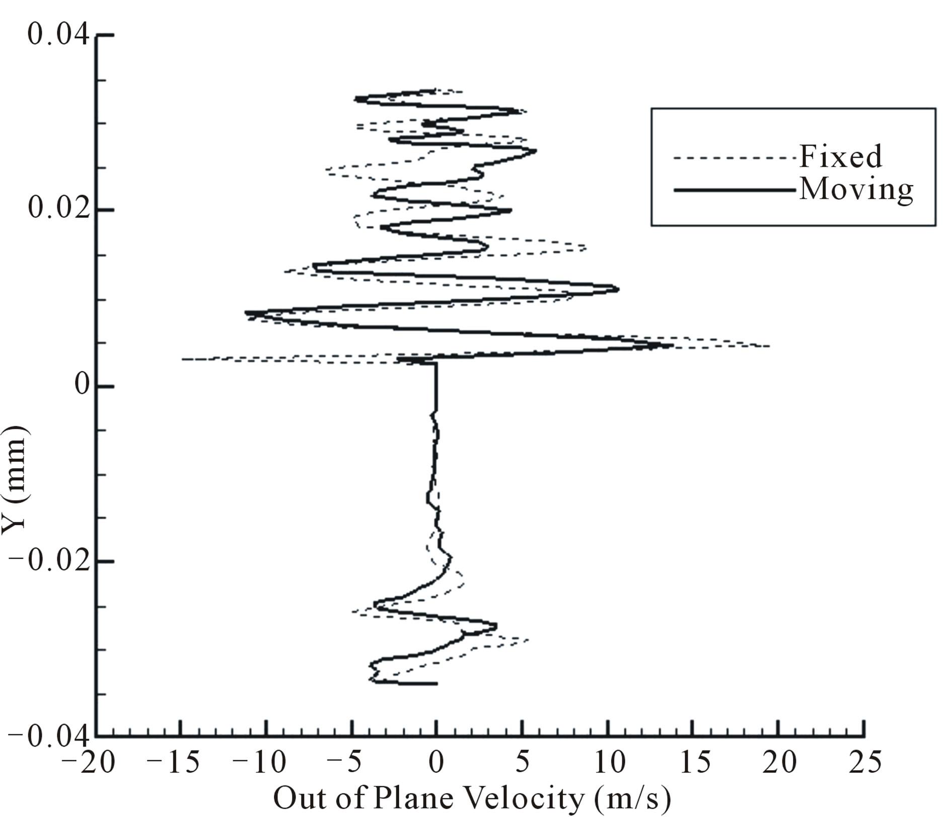
Figure 9.Comparison plot of Y axis vs. out of plane velocity at Z = 9.725 mm, X = 34 mm.
plitude against initial as 1194/1800 = 0.663. The value of 0.663 represents an approximate converged figure. A round-off figure of 0.65 is finally chosen here and applied to the 3.5 inch HDD by assuming the structure dynamics is statistically similar between them.
3. Application of Simulated Results on the Actual 3.5 Inch HDD
We aim to obtain a benchmark parameter that could be easily applied by the electronics industry in the research and development of HDDs. The parameter is the ratio of the moving HSA vibration against static HSA vibration. This parameter would be useful in allowing hard disk manufacturers to simulate the vibration of the HSA relatively accurately without going through the lengthy process of performing the detailed FSI study.
The simulation approach in deriving the parameter involves:
1) Run 5000 steps of FLUENT k-ε transient simulation 2) Run 5000 steps of LES with moving HSA, applying the 0.65 ratio obtained from the previous FSI study on a 3.5 inch HDD simulation. HSA is modeled to vibrate in FLUENT through the use of UDF.
3) Transfer forces on all nodes on the HSA over to the structural model.
4) Solve the structural components using ANSYS.
5) Analyze results to obtain benchmark parameter.
The equation that controls the velocity of the HSA’s vibrations is derived (same approach as Equation (7)) as follow:
 (8)
(8)
where,
 and
and  .
.
Figure 10 shows detail layout (CAD, mesh, location of sliders) of the 3.5 inch HDD and the HSA being investigated.
The Kolmogorov length scale is given as follows:
 (9)
(9)
While the Kolmogorov time scale is:
 (10)
(10)
As the length scale is very small, limitations in computational resources available make such a small scale challenging and unachievable. Hence the authors have performed a mesh dependence study as detailed in Section 2.2. The mesh for this study and the FSI study of a 3.5 inch HDD is created based on the results from Section 2.2 instead of using the Kolmogorov length scale.
The time scale is achievable and hence would be used for this study.
The stated case setup has Re = 22.97 × 10⁴ with turbulent flow and was setup to run RNG k-ε (5000 iterations) followed by LES (5000 time steps, step size = 2 × 10⁻⁶ & 5 iterations per step).
The force extraction methodology is similar to that described in Section 2.4.2. In total, 20000 time steps of force data were extracted. The material properties for the structural model are included in Table 6.
Figure 11 shows the graph of standard deviation of displacement against slider for the four cases, fixed HSA, moving HSA, 65% of fixed HSA and the average between the 65% and moving HSA results respectively. Fixed HSA refers to the HSA being modeled as an assembly that does not vibrates on its own, but is affected by the surrounding air flow. Moving HSA refers to the HSA being subjected to a vibration amplitude and frequency as described by the formula in Equation (3). The 65% of fixed HSA line represents the displacement of fixed HSA multiplied by a factor of 0.65. This line is meant to be used as a comparison against the moving HSA line.
It can be seen from Figure 12 suggests that the displacement for moving HSA is significantly lower than that of fixed HAS as expected. A fixed HSA would provide a greater amount of resistance to the surrounding air flow, leading to a greater force applied on it, and hence larger displacement. However, this would be an inaccurate case of the actual situation that is happening within the HDD. This is because the HSA of the HDD is actually vibrating instead of being rigidly fixed. Hence a model which considers the HSA to be rigidly fixed would result in the HSA facing higher forces, and thus higher vibration amplitudes.
From Figure 11, the calculated force for the moving HSA is about 26.5% less than that of fixed HSA. This is a very significant difference, and it implies that a hard disk designer who bases his/her design on simulation results of fixed HSAs values would yield inaccurate results. The average of the 65% and moving HSA results is about 69% of the fixed HSA results. The authors propose that future researchers who are unable to commit the time and/or resources to perform a full FSI analyses of their
 (a)
(a)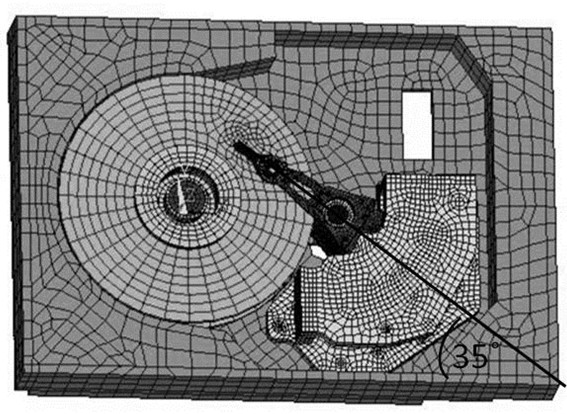 (b)
(b) (c)
(c)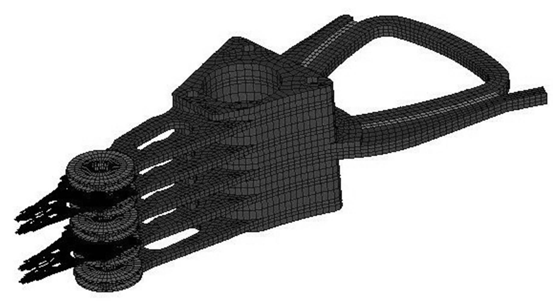 (d)
(d)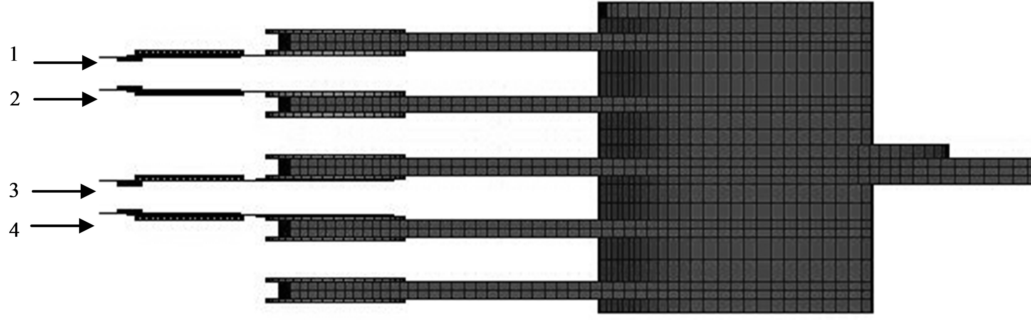 (e)
(e)
Figure 10. Details of 3.5 inch HDD Assembly. (a) CAD model of 3.5 inch HDD; (b) Structural model of 3.5 inch HDD(c) CAD drawing of HAS; (d) Structural model of HAS; (e) Structural model of HAS: side view depicting location of sliders.

Table 6.Material properties used for 3.5 inch HDD model.
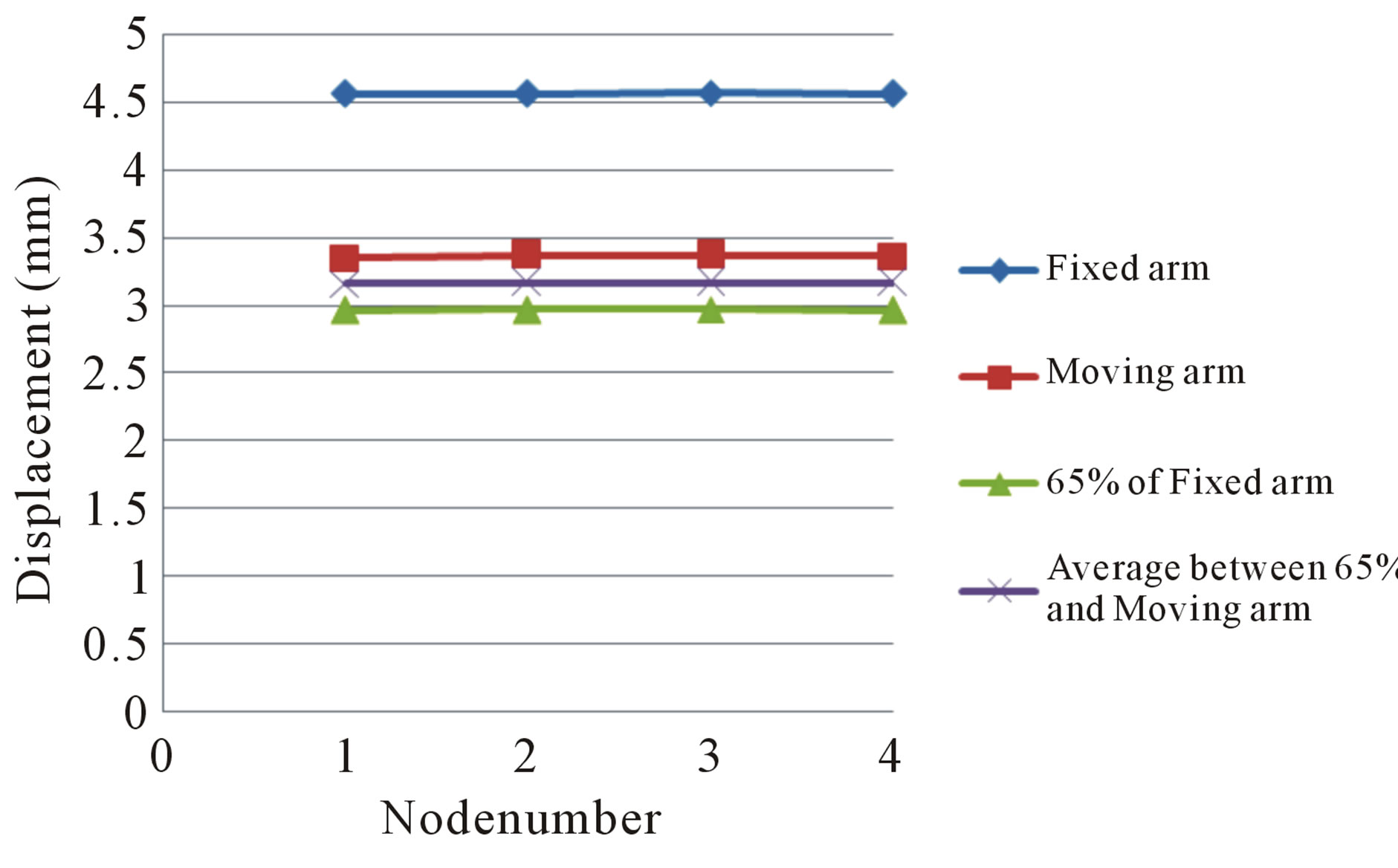
Figure 11.Standard deviation of displacement vs. slider number (Z direction) for 3.5 inch HDD’s HAS.
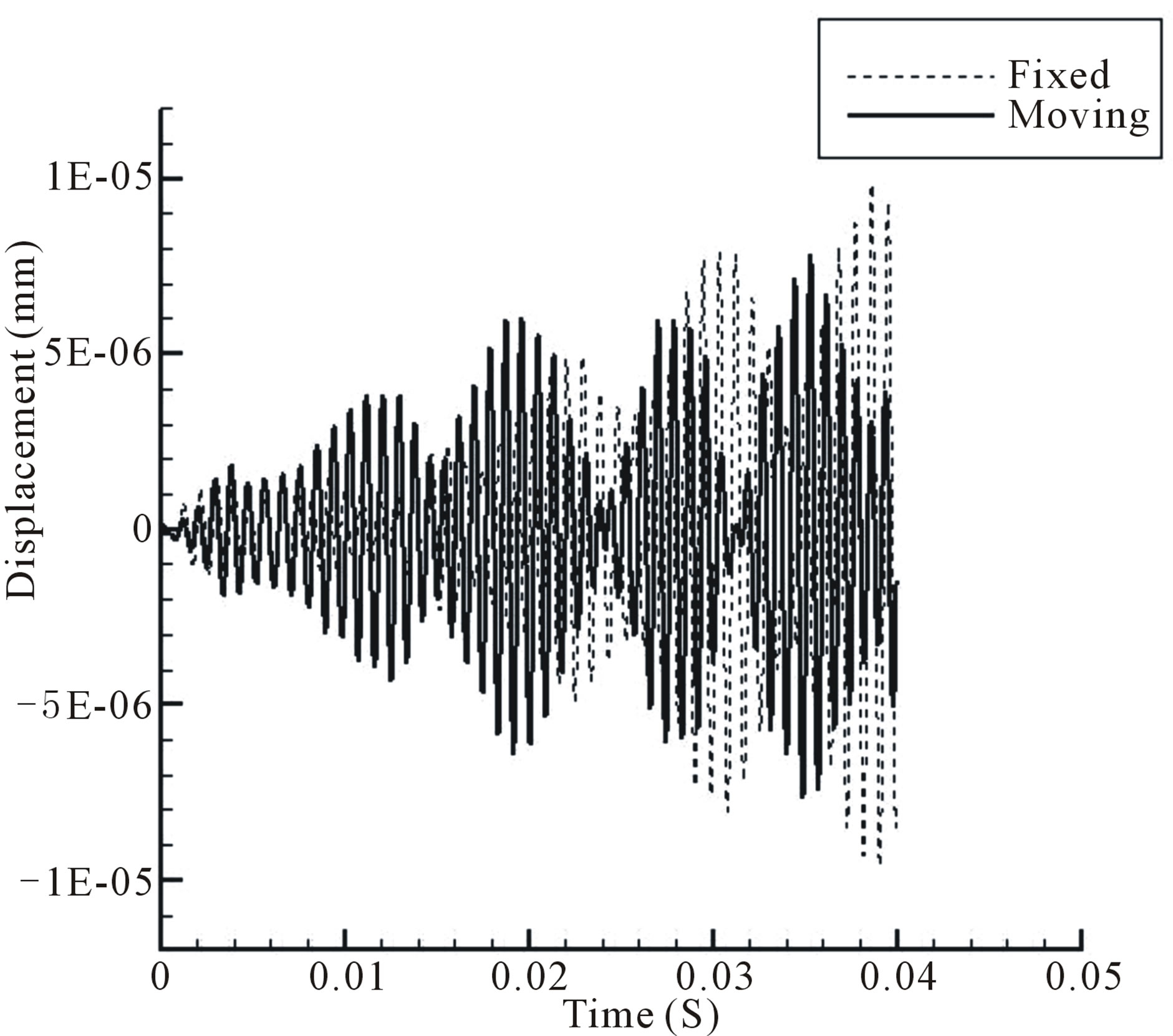
Figure 12.Slider 2 vibration: comparison of fixed and moving HSA cases.
HDD may adopt this 69% value in their design work. This 0.69 ratio would allow engineers to quickly and relatively accurately understand the vibration of the HSA by just performing a fixed HSA case of their hard disk. The 0.69 ratio would represent a situation that is 31% more accurate than a fixed HSA [10], when applied on 3.5 inch HDDs at 15000 rpm.
By observing Figure 11, one can tell that the magnitude of the standard deviations do not vary much across the 4 sliders and the magnitudes at sliders 2 and 3 are higher than those of sliders 1 and 4, albeit only slightly. This is within expectations as HSA 1 and 4 are closer to the top and bottom walls of the HDD, hence the air flow should be slower, resulting in smaller vibration of the HSAs.
Figure 12 shows the differences in vibration between the fixed HSA and moving HSA for slider 2. Slider 3 has a very similar trend as slider 2 (i.e. reaching a statistically steady state) and the plot is thus not shown here. The displacement for both fixed HSA and moving HSA follow a similar basic shape of starting off small and then progressively becomes larger. However the displacement for fixed HSA starts off smaller and seems to lag behind moving HSA in its cycles. The fixed HSA’s displacement magnitude becomes significantly larger than the moving HSA from about 0.25 s onwards, even though it still seems to lag behind moving HSA.
These observations make sense. For the moving HSA case, the HSA is made to vibrate based on the Equation (8). It would vibrate even without any interaction with the surrounding air flow, causing the initial displacement to be larger than the fixed HSA case. But when the disk begins to rotate, the rotating air flow would interact with the vibrating HSA, leading to increases in displacement.
However for the fixed HSA case, the HSA is assumed to be fixed, and vibrates due to interactions from the surrounding air flow. It starts off like a “barrier” to air flow, causing its initial displacement to be much smaller than the moving HSA case. It blocks the surrounding air flow and hence the air flow would impart large forces on it, causing its’ displacement to become larger, eventually surpassing the displacement of the moving HSA case.
Figure 13 shows the out of plane velocity contours (at Z = 7.6 mm) of both the fixed and moving HSAs. It can be noted that the differences in the two contours are very slight. This is within expectations as the turbulent flow within the HDD is very complex due to the complex geometry of the HDD. Moreover, the HSA is placed at an angle of 35˚ with respect to the longest side (length) of the HDD, which results in the nano-scale movement of the HSA to have very little impact on the general flow field within the HDD.
In summary, it can be observed that the fixed HSA case vibrates in the out of plane direction with greater displacement and velocity. During numerical simulation, a researcher that models the HSA as a fixed HSA would obtain inaccurate results. In particular, the out of plane vibration amplitudes and velocities would be far too
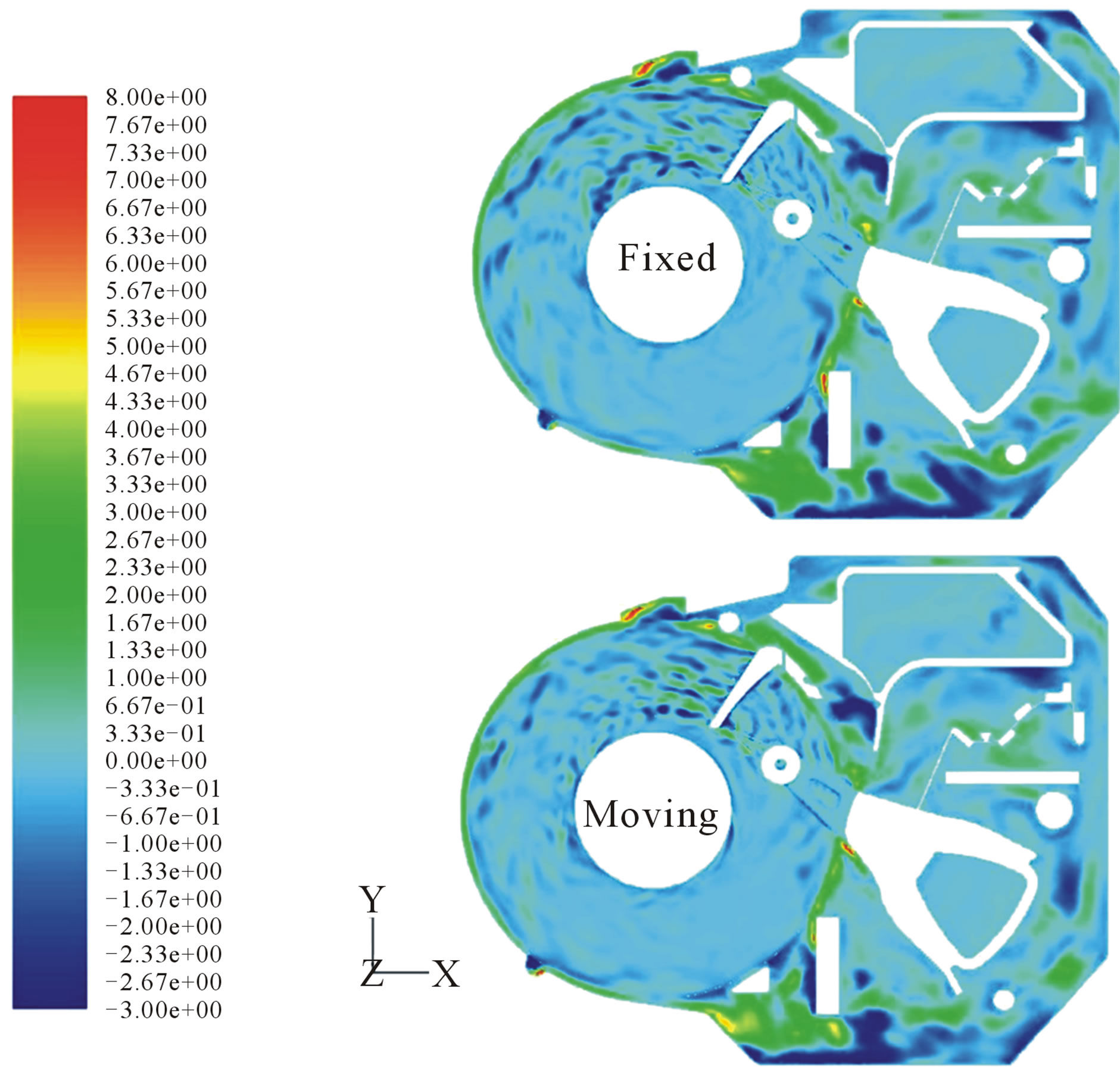
Figure 13.Comparison of fixed and moving HSA out of plane velocity (m/s) contour, at Z = 7.6 mm.
large. In addition, the vibration of a fixed HSA would also lag that of a moving HSA. Hence, engineers designing the damping and controls of the HDD might not achieve the best results if they were to base their analysis on a fixed HSA case.
4. Conclusions
This paper was to develop a novel method for performing FSI studies for HDD by utilizing a weak coupling method where the fluid and structural components are solved sequentially. This method allowed the authors to propose a benchmark parameter for future researchers to utilize. This benchmark index is 0.69 (though not universal), and it may represent the ratio of the out of plane displacement amplitude between the fixed and moving HSA. This parameter may allow future researchers to quickly model the out of plane vibrations of a HSA without performing a detail FSI study. Researchers that model their HSA as a fixed HSA would overrate the vibrations of the HSA, leading to inaccurate results. This new method would reduce overrating through the use of this benchmark parameter. Though it might be more expensive than the weak coupling used in the paper, the accuracy of the results must be validated using the strong coupling form as future work.
Vibration of the HSA was modeled through the use of an equation, with the frequency and initial amplitude obtained from a fixed HSA case. The results showed that the out of plane amplitude and velocity of the fixed HSA’s case is higher than the moving HSA case. We applied the 0.65 benchmark parameter obtained from the previous study for a real 3.5 inch HDD. This may enable us to study the effects of applying this parameter, and propose a final benchmark parameter that achieves a 31% more accurate simulation of out of plane HSA vibrations for 3.5 inch HDDs at 15000 rpm and hence assisting in the development of better HDDs.
REFERENCES
- R. Kral and E. Kreuzer, “Multibody Systems and FluidStructure Interactions with Application to Floating Structures,” Multibody System Dynamics, Vol. 3, No. 1, 1992, pp. 65-83. doi:10.1023/A:1009710901886
- S. Badia and R. Codina, “On Some Fluid-Structure Iterative Algorithms Using Pressure,” International Journal for Numerical Methods in Engineering, Vol. 72, No. 1, 2007, pp. 46-71. doi:10.1002/nme.1998
- Q. Zhang and T. Hisada, “Studies of the Strong Coupling and Weak Coupling Methods in FSI Analysis,” International Journal for Numerical Methods in Engineering, Vol. 60, No. 12, 2004, pp. 2013-2029. doi:10.1002/nme.1034
- V. Sankaran, J. Sitaraman, B. Flynt and C. Farhat, “Development of a Coupled and Unified Solution Method for Fluid-Structure Interactions,” Springer, Berlin, 2009.
- C. Liang, R. Kannan and Z. Wang, “A p-Multigrid Spectral Difference Method with Explicit and Implicit Smoothers on Unstructured Triangular Grids,” Computers and Fluids, Vol. 38, No. 2, 2009, pp. 254-265. doi:10.1016/j.compfluid.2008.02.004
- R. Kannan and Z. Wang, “A Study of Viscous Flux Formulations for a p-Multigrid Spectral Volume Navier Stokes Solver,” Journal of Scientific Computing, Vol. 41, No. 2, 2009, pp. 165-199. doi:10.1007/s10915-009-9269-1
- C. Bernardo and C. W. Shu, “The Runge-Kutta Discontinuous Galerkin Method for Conservation Laws V: Multidimensional Systems,” Journal of Computational Physics, Vol. 141, No. 2, 1998, pp. 199-224.
- ANSYS Fluent Software, 2011. http://www.ansys.com/About+ANSYS
- K. Aruga, M. Suwa, K. Shimizu and T. Watanabe, “A Study on Positioning Error Caused by Flow Induced Vibration Using Helium-Filled Hard Disk Drives,” IEEE Transactions on Magnetics, Vol. 43, No. 9, 2007, pp. 3750-3755. doi:10.1109/TMAG.2007.902983
- N. Liu, Q. D. Zhang and K. Sundaravadivelu, “A New Fluid Structure Coupling Approach for High Frequency/ Small Deformation Engineering Application,” Asia-Pacific Magnetic Recording Conference, Singapore, 10-12 November, 2010, pp. 1-2.
- J. Videler, “Fish Swimming,” Chapman & Hall, London, 1993. doi:10.1007/978-94-011-1580-3
NOTES
*Corresponding author.