World Journal of Condensed Matter Physics
Vol.3 No.3(2013), Article ID:35302,8 pages DOI:10.4236/wjcmp.2013.33022
Chaos Appearance during Domain Wall Motion under Electronic Transfer in Nanomagnets
![]()
Fundamental Physics’ Laboratory, Group of Nonlinear Physics and Complex System, Department of Physics, Faculty of Science University of Douala, Douala, Cameroon.
Email: nguenang@yahoo.com
Copyright © 2013 Donfack Gildas Hermann, Jean-Pierre Nguenang. This is an open access article distributed under the Creative Commons Attribution License, which permits unrestricted use, distribution, and reproduction in any medium, provided the original work is properly cited.
Received December 27th, 2012; revised May 27th, 2013; accepted June 11th, 2013
Keywords: Domain Wall Motion; Magnetization Dynamics; Chaos Appearance
ABSTRACT
In this paper, we study the likelihood of chaos appearance during domain wall motion induced by electronic transfer. Considering a time-varying current density theory, we proceed to a numerical investigation of the dynamics. Using the dissipation parameter, amplitude and frequency of current density as control parameters; we show how periodic regime as well as chaotic regime can be exhibited in nanomagnetic systems. Numerical results allow setting up the periodicity and quasi-periodicity of system and chaotic phenomena occurring during magnetization switching process in nanomagnet through electronic transfer.
1. Introduction
Since the appearance of pioneering work done by Berger [1,2] and Slonczewski [3], considerable progress has been made in understanding current-induced domainwall (DW) dynamics in ferromagnetic strips [4-8]. The key mechanism is that of a spin torque resulting from a spin-polarized current passing through a DW where the spin of the itinerant conduction electron, couples to the local spatial gradient of the magnetization. The integration of magnetization and electric properties is very important in the present technological context, where most of magnetic device are nowadays based on the magnetoresistive effect arising from the modification of the electron transport by the magnetic configuration. The manipulation of magnetization by the use of electric current is singularly promising for the new and next generation of magnetic memories for which information can be written by electric current.
Nowadays, it is well known that the concept and methods for the theory of nonlinear processes have substantially enriched many fields of physics, such as from elementary particle physics to biophysics, to mention just a few. An important field in nonlinear physics is the study of chaos in various dynamical systems [9]. In many systems, chaos is not associated with the presence of any random parameters and forces but is reader due to the unstable character of the trajectories in phase space. Chaos can actually be very useful under some circumstances, for example, in encryption, digital communications, etc. So, chaotic system is very important in such engineering application.
The aim of this paper is to investigate the phenomenon of chaos in a nanomagnetic (spin) system under electronic transfer. It is important to understand the behavior of domain-wall (DW) whose dynamic, may depend not only on an induced-current through electron motion or either on an applied field but also on the fundamental characteristics of metal. Such chaos investigation may lead to dynamical characterization of such system that are of great importance for determining the suitable parameters for magnetic storage of nanomagnets. Probing the influence of each parameter on the DW motion may help in determining the spin switches behavior which is one of the key processes in reading and writing for magnetic memories devices.
Before pursuing, one should keep in mind that the damping parameter doesn’t only influence the nature of motion; it is rather a key parameter that is responsible for chaos appearance as current density amplitude and current density frequency in the system as shown in this paper.
The first experimental evidence of low-current operation due to the resonant DW motion induced by oscillating currents was carried out by Saitoh et al. [10]. Motived by this observation, Tatara et al. [11,12] studied the response of a pinned DW inside a parabolic potential subjected to the action of oscillating current density in ferromagnetic films loaded in a xy-plane with easy axis z. Using a deterministic one-dimensional description, they showed that the DW depinning occurs at a density current, which is lower than the dc case if the frequency is tuned close to the pinning frequency. Other experimental confirmation of this theoretical prediction was done by Thomas et al. [13,14]. Using a train of current pulses with zero rise and fall times, they showed that the DW depinning can be efficiently achieved if the lengths and separation of the pulses are tuned to the characteristic pinning period.
In the present work, time-varying electrical density current in the form  is applied along with j0 being the amplitude of the current’s density and w0, is the frequency of oscillation.
2. Model and Modeling
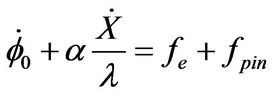
We consider a ferromagnet consisting of localized spins and conduction electrons. The spins are assumed to display an easy axis and a hard axis. In the continuum approximation, considering harmonic pinning potential, while assuming to work in the framework of a one dimensional spin lattice, the equation of motion of the wall we consider is given by [7]:
 (1)
(1)
 (2)
(2)
where
 (3)
(3)
and
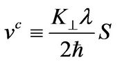 (4)
(4)
 has the dimension of velocity. The equations of motion in terms of dimensionless parameters are given by [15,16]:
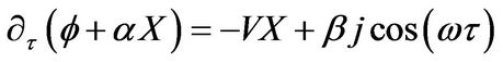 (5)
(5)
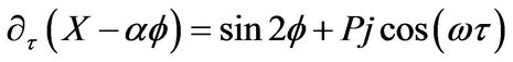 (6)
(6)
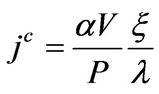
where ; t is time parameter,
 ; X position of the domain wall center and λ the wall width parameter,
  where p is the spin current polarization and S spin magnitude,
 ; j0 is current density amplitude is
  where V0
pinning potential magnitude and ξ is the width of pinning potential, .
.
By eliminating  from the previous Equations (2) and (3) we obtain the following dynamical equation in function of the angle ϕ shown in Figure 1, which is the equation governing the DW:
 (7)
(7)
where β is the non-adiabatic parameter, P is the spin current polarization. Considering a Taylor development around; we obtain the magnitude of transfer function given by:
 (8)
(8)
The parameters ωn and ζ are the angular corner frequency of DW and damping factor, respectively defined by:
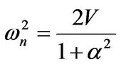 (9)
(9)
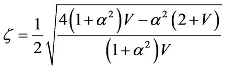 (10)
(10)
The resonance angular frequency is the minimum of the square of denominator transfer function denoted by η(ω) as:
 (11)
(11)
In this framework, we determine the resonance angular frequency.
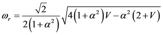 (12)
(12)
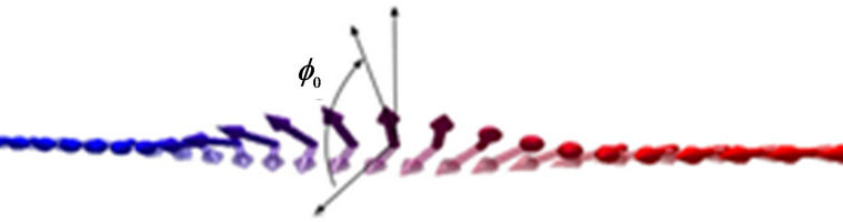
Figure 1. Domain wall configuration where the easy axis is along the wall direction, so called the Néel wall. The angle out of the easy plane is ϕ. which a canonical momentum of the wall is of great importance in the DW dynamics. The dynamics of ϕ (named the chirality of the wall) is discussed in Refs [17,18].
Since the resonance frequency corresponds to the highest displacement of the domain wall, the frequency of the current density has to be chosen taking into account the resonance frequency to keep the wall safe. In this respect, to avoid the highest vibration of the wall, the frequency of the current density has to be less than the resonance frequency.
3. Numerical Experiment
The numerical investigation has been done while using a Matlab software in addition Fortran 90 codes. The outcomes were obtained by solving equation (7) with help of the standard fourth-order Runge-Kutta algorithm (Matlab’s ode45). For more detail concerning DW dynamics we have proceed to a meticulous bifurcation analysis.
Domain Wall Bifurcation
A Bifurcation analysis is always useful and it is a widely studied subfield of dynamical systems. The observation of the bifurcation scenario allows one to draw qualitative and quantitative conclusions about the structure and dynamics of a given system. Several problems have been investigated using such a theoretical approach.
In the numerical results that follow, we investigate the dependence of the DW behaviour on the dissipation parameters α. Here, the amplitude of the current density  and the frequency of the current’s density are used as the control parameters.
While looking at Figure 2, it is important to notice that from this plot of the numerical computation of the velocity of the wall as function of the frequency, the motion of DW depends on frequency of the current’s density [4,15]. The depinning threshold is much lower when an ac current is applied than the dc case. The threshold current in dc case is given by:
 (13)
(13)
for . In this specific case (time varying current density), the threshold is lower as shown in Figure 2. The DW is depinned for the current density in the range
 .
.
It is worth mentioning the fact that the bifurcation diagram presented here consists of a projection of the attractors in the phase space into one of the DW coordinates versus α. To gain further insight on the dynamics of the equation under investigation, we compute the phase space and a Lyapunov spectrum (Lya). These results are obtained solving equation (7) with the help of the standard fourth-order Runge-Kutta algorithm.
Figure 3 shows the outcome of the computation of the bifurcation diagram from which a Lyapunov spectrum is set up as exemplified in Figure 4. From these later fig-

Figure 2. Domain wall velocity  versus current density (j) in the case of β = 0.001 where f = 2.5 (magenta) f = 5 (blue). Finite threshold appears due to intrinsic pinning due to the frequency of current.
Figure 3. Bifurcation diagrams. Position ϕ versus damping parameter α for pinning potential V = 1200 with j = 0.906 and f = 5. Periodic windows sandwiched by chaotic domains, a sequence of reverse periodic-doubling route to periodic regime are also visible.

ures it is realized that for the parameter region ranged from α = 0.017 to α = 0.0185, the Feigenbaun scenario is exhibited by the period doubling bifurcation. This is almost known as one of the routes toward chaos in this system [19]. The existence of Lyapunov function is sufficient to characterize the stability or the instability in the system since their signature is ruled by the sign of the Lyapunov parameter (Lya). If the parameter, Lya is negative, then the system undergoes a stable state (periodic or quasi-periodic motion) and it becomes chaotic if Lya becomes positive. For α < 0.01722, we find chaotic orbits of the DW behavior. In the periodic window 0.0173 ≤ α ≤ 0.01872, a sequence of reverse periodic-doubling bifurcations yields a period-5 attractor which is later destroyed for α = 0.01873 in a crisis event. This can be understood as a sudden chaos occurring in the system. After the large chaotic domain intermingled with windows made up of periodic orbits, another reverse periodicdoubling occurs for 0.0198 ≤ α < 0.02 and become instantly periodic. This bifurcation scenario is in fact the feature of the dynamics of the spin system as far as α is further increased. However, for α > 0.0202, we find periodic orbits dominating the domain-wall motion. Notice that bifurcation observed throughout this study is perfectly traced by the Lyapunov spectra. Figure 5 is constituted with plots of the phase space, which is the space of all possible states of the underlying dynamics of the physical system. It corresponds to bifurcation diagram (see Figure 3) and Lyapunov spectrum (see Figure 4). In this respect, one needs both the position and speed of a given system in order to determine the phase space [20]. A strange attractor is characterized by movements reaching to a steady state or reproduce indefinitely. Figure 5(a) displays a strange chaotic attractor for α = 0.0172, during the transition for which the domain wall motion moves away from the attracting period-6 invariant closed curve for α = 0.01725 as seen in Figure 5(b). Figure 5(c) shows period-3 for α = 0.01725, then after large values of α, the domain wall motion becomes periodic (see Figure 5(d)).
Figure 6 obtained for α = 0.02 and j = 5.7, displays the bifurcation diagram of domain wall position versus current density frequency f. It can be realized while looking at Figure 6 that there are periodic, quasi-periodic windows and chaotic regions occurring alternatively when the frequency is in the range of . This period-doubling scenario is indeed the road towardschaos as previously mentioned. Figure 7 shows the phasespace trajectories that are constituted by the velocity (ϕ) versus position (ϕ). It displays the explicit bifurcation from the periodic motion of the underlying spin system with period-4 to the chaotic motion that is more close to
 (a)
(a)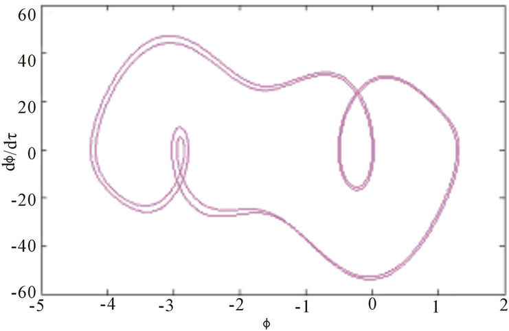 (b)
(b) (c)
(c)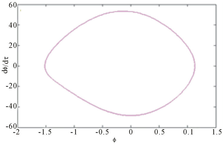 (d)
(d)
Figure 5. Phase space ϕ vs ϕ illustrating the supercritical bifurcation for f = 5 and j = 0.906: (a) α = 0.017, (b) α = 0.01725, (c) α = 0.0173, (d) α = 0.0205.
a chaotic strange attractor. The Poincare section extends our investigations. This technique is particularly suited to the study of periodic system since it clearly distinguishes the quasi-periodic regimes of chaotic system. The poincare section is defined by the set of points of intersection of a plane with the trajectory of the state vector in space. Figure 8 shows the Poincare section, it corresponds to a chaotic behavior seen in Figure 7(a). Needless to mention is the fact that the DW motion can be classified in a periodic regime if the frequency is realized in the range of .
.
Figure 9 shows the bifurcation diagram of domain wall position versus current density amplitude j. Here it is plotted in a large window between 4 and 7.5 but to illustrate the behavior of the domain wall out of this window, we just zoom the window between 7.02 and 7.11. From this figure, it is realized that there are many period and period-doubling windows between chaotic regions. The Poincaré section of trajectory is shown in Figure 10. Figure 10(a) corresponds to a strange attractor for j = 5.7. In this case strong oscillations of the wall occur. Figure 10(b) corresponds to a periodic-3 domain-wall motion. Next, we focus our interest on Figures 11 and 12. They show the diagram of Figure 8 for the region expanded from j = 7.01 to 7.11 and j = 7.18 to 7.27 respectively. Outside this region, when j ≤ 7.01 the system is chaotic and for j ≥ 7.27, it returns to a periodic regime. Here, the Feigenbaun scenario by period doubling bifurcation is found to be one of the roads to chaos in this system [19-21].
While looking at Figure 13, it is realized that the instability of domain-wall is characterized by changes in the real-time signals of the wall vibrations from periodic to chaotic motion.
The Poincaré section of the phase trajectory is shown in Figure 14. It corresponds to periodic motion for Figure 14(a), but to periodic-2 in the case of Figure 14(b)in Figure 14(c), it corresponds to a periodic-4 motion and periodic-8 for the case of Figure 14(d) as showed by bifurcation diagram. This is an example of the Feigenbaun scenario displayed once more by the underlying spin dynamics [19-21].
From the results of the study of chaos in this ferromagnetic system, we realized that it is of capital interest and in this respect it deserves a peculiar attention. The above outcome shows the periodicity and unpredictability of DW motion for some values of control parameters where the system falls into periodic or chaotic, regime. We consider the physical value given by [15]. The anisotropy of energy is  and using
 ,
, 
and λ = 70 nm. By considering these parameters the resonance frequency is fc = 2.5 GHz. When the wall moves periodically, in a chosen phase subspace such a motion corresponds to the point attractor. In this case the Bloch surface of the wall is uniform and therefore the spin switches can be proceed successively. Chaotic motion corresponds to a strange attractor in the phase space. In this case, the strong oscillations of the wall occur.

Figure 6. Bifurcation diagram. Position ϕ varying with current frequency f for α = 0.02 and j = 5.7.
 (a)
(a) (b)
(b)
Figure 7. Phase space (velocity  versus position ϕ) for α = 0.02, j = 5.7: (a) chaotic orbit f = 6.025; (b) period-4 orbit f = 5.15.
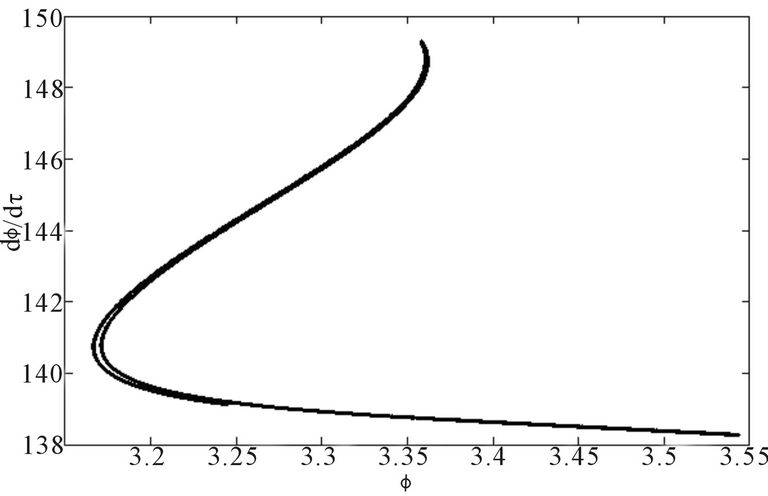
Figure 8. Poincare section (velocity  versus position ϕ) for α = 0.02, j = 5.7: chaotic orbit f = 6.025.

Figure 9. Bifurcation diagram. Position ϕ varying with current density j for α = 0.02 and f = 6.025.
 (a)
(a)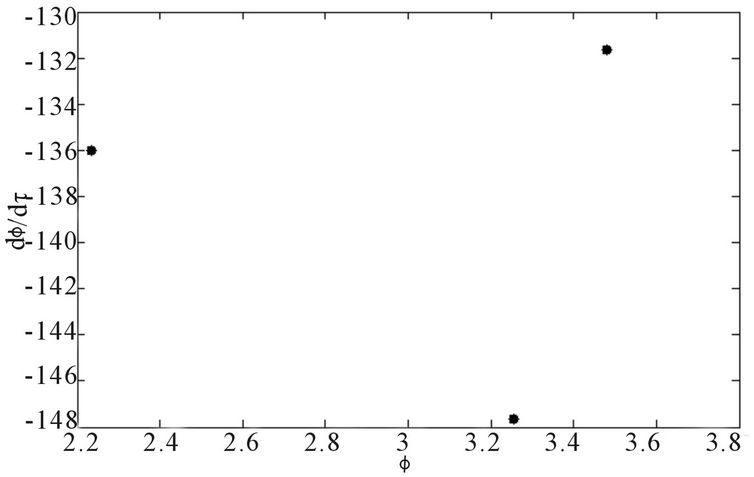 (b)
(b)
Figure 10. Poincare section (velocity  versus position ϕ) for α = 0.02, f = 5.002: (a) chaotic orbit j = 4.2; (b) 3-period orbit j = 4.4.

Figure 11. Bifurcation diagram. Position ϕ varying with current density j for α = 0.02 and f = 5.002.
The amplitude of these oscillations is of order of π. This means that the vertical Bloch lines are generated in the wall and therefore the switching process occurs randomly [20].
The knowledge of this unpredictable behavior of the DW motion is very important in technology based on the switching processes. It is clear that such a study would

Figure 12. Bifurcation diagram. Position ϕ varying with current density j for α = 0.02 and f = 5.002.
help in determining suitable range of parameter for the safe and sustainable switching process, which is of outmost importance for magnetic recording technology.
4. Concluding Remarks
In summary, we have introduced a model of periodically time-varying current density. We have shown that the
 (a)
(a) (b)
(b)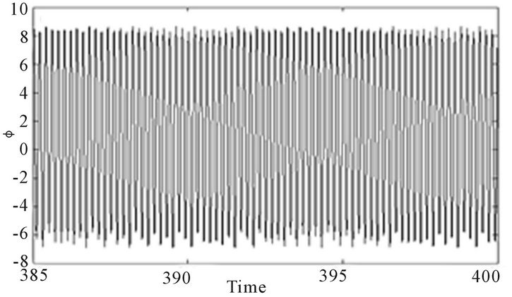 (c)
(c) (d)
(d)
Figure 13. Temporal space (position ϕ versus time τ) and Phase space (velocity  versus position ϕ) for α = 0.02, f = 5.002: (a) period-2 orbit j = 7.06; (b) period-4 orbit j = 7.09; (c) period-2 orbit j = 7.11; (d) chaotic orbit j = 7.11.
 (a)
(a) (b)
(b)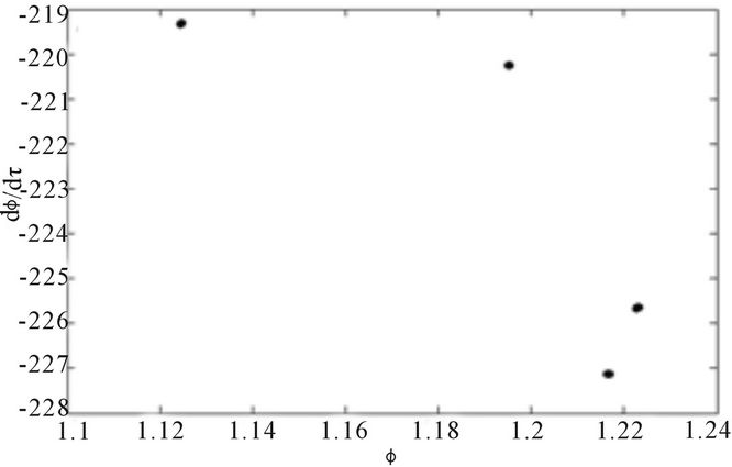 (c)
(c)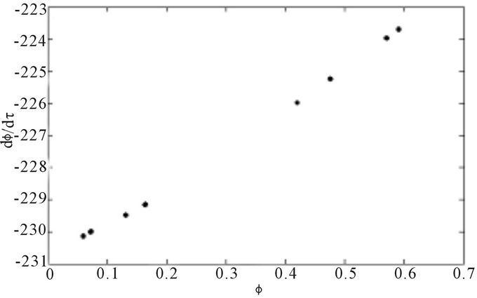 (d)
(d)
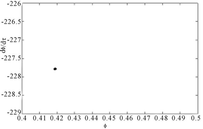
Figure 14. Poincare section (velocity  versus position ϕ) for α = 0.02, f = 5.002: (a) 1-period orbit j = 7.27; (b) 2-period orbit j = 7.23; (c) 4-period orbit j = 7.21; (d) 8-period orbit j = 7.20.
model admits a very complex dynamical structure that strongly depends on the control parameters. Using a phase space diagram; periodic, quasiperiodic and chaotic attractors of the DW motion were presented, setting then up three different regimes of spin switches when a nano-magnet undergoes an electronic transfer. Furthermore, the structures found in this model can be perfectly traced by the Lyapunov spectrum. This spectrum shows spikes at the bifurcation point reflecting a sudden change in the system. The outcomes of this work are element of an important step toward determining chaos in magnetic nanowire. However, further studies are necessary for controlling possible chaos in the system. Hence, further numerical and experimental investigations are encouraged.
REFERENCES
- L. Berger, “Low-Field Magnetoresistance and Domain Drag in Ferromagnets,” Journal of Applied Physics, Vol. 49, No. 3, 1978, pp. 2156-2161. doi:10.1063/1.324716
- L. Berger, “Exchange Interaction between Ferromagnetic Domain Wall and Electric Current in Very Thin Metallic Films,” Journal of Applied Physics, Vol. 55, No. 6, 1954.
- J. C. Slonczewski, “Excitation of Spin Waves by an Electric Current,” Journal of Magnetism and Magnetic Materials, Vol. 195, No. 2, 1999, pp. L261-L268. doi:10.1016/S0304-8853(99)00043-8
- G. Tatara and H. Kohno, “Theory of Current-Driven Domain Wall Motion: Spin Transfer Versus Momentum Transfer,” Physical Review Letters, Vol. 92, No. 8, 2004, Article ID: 086601. doi:10.1103/PhysRevLett.92.086601
- S. E. Barnes and S. Maekawa, “Current-Spin Coupling for Ferromagnetic Domain Walls in Fine Wires,” Physical Review Letters, Vol. 95, No. 10, 2005, Article ID: 107204. doi:10.1103/PhysRevLett.95.107204
- A. Yamaguchi, T. Ono and S. Nasu, “Real-Space Observation of Current-Driven Domain Wall Motion in Submicron Magnetic Wires,” Physical Review Letters, Vol. 92, No. 7, 2004, Article ID: 077205. doi:10.1103/PhysRevLett.92.077205
- N. Vernier, D. A. Allwood, D. Atkinson, M. D. Cooke and R. P. Cowburn, “Domain Wall Propagation in Magnetic Nanowires by Spin-Polarized Current Injection,” Europhysics Letters, Vol. 65, No. 4, 2004, pp. 526-532. doi:10.1209/epl/i2003-10112-5
- D. Bouzidi and H. Suhl, “Motion of a Bloch Domain Wall,” Physical Review Letters, Vol. 65, No. 20, 1990, pp. 2587-2590. doi:10.1103/PhysRevLett.65.2587
- K. N. Aleskseev, G. P. Berman, V. I. Tsifrinovich and A. M. frishman, “Dynamical Chaos in Magnetic Systems,” Soviet Physics Uspekhi, Vol. 35, No. 7, 1992.
- E. Saitoh, H. Miyajima, T. Yamaoka, and G. Tatara, “Current-Induced Resonance and Mass Determination of a Single Magnetic Domain Wall,” Nature, Vol. 432, No. 7014, 2004, pp. 203-206. doi:10.1038/nature03009
- G. Tatara and H. Kohno, “Microscopic Theory of Current-Driven Domain Wall Motion,” Journal of Electron Microscopy, Vol. 54, No. 1, 2005, pp. i69-i74. doi:10.1093/jmicro/54.suppl_1.i69
- G. Tatara, E. Saitoh, M. Saitoh, M. Ichimura and H. Kohno, “Domain-Wall Displacement Triggered by an ac Current Below Threshold,” Applied Physics Letters, Vol. 86, No. 23, 2005, Article ID: 232504. doi:10.1063/1.1944902
- E. Martinez, et al., “Resonant Domain Wall Depinning Induced by Oscillating Spin-Polarized Currents in Thin Ferromagnetic Strips,” Physical Review B, Vol. 77, No. 14, 2008, Article ID: 144417. doi:10.1103/PhysRevB.77.144417
- L. Thomas, M. Hayashi, X. Jiang, R. Moriya, C. Rettner and S. S. P. Parkin, “Resonant Amplification of Magnetic Domain-Wall Motion by a Train of Current Pulses,” Science, Vol. 315, No. 5818, 2007, pp. 1553-1556. doi:10.1126/science.1137662
- G. Tatara, H. Kohno, J. Shibata, “Recent Developments in Theory of Current-Induced Domain Wall Dynamics,” Physics Reports, Vol. 468, 2008.
- G. Tatara, T. Takayama, H. Kohno, J. Shibata, Y. Nakatani and H. Fukuyama, “Threshold Current of Domain Wall Motion under Extrinsic Pinning, β-Term and NonAdiabaticity,” Journal of the Physical Society of Japan, Vol. 75, 2006, Article ID: 064708. doi:10.1143/JPSJ.75.064708
- H. B. Braun and D. Loss, “Berry’s Phase and Quantum Dynamics of Ferromagnetic Solitons,” Physical Review B, Vol. 53, No. 6, 1996, pp. 3237-3255. doi:10.1103/PhysRevB.53.3237
- S. Takagi and G. Tatara, “Macroscopic Quantum Coherence of Chirality of a Domain Wall in Ferromagnets,” Physical Review B, Vol. 54. No. 14, 1995, pp. 9920-9923. doi:10.1103/PhysRevB.54.9920
- H. Okuno, Y. Sugitani and K. Hirata. “Bifurcation Diagram and Power Spectrum of Chaotic Domain-Wall Motion,” Journal of Magnetism and Magnetic Materials, Vol. 140-144, 1995, pp. 1879-1880. doi:10.1016/0304-8853(94)00927-9
- R. A. Kosinski and A. Sukiennicki. “Chaotic Motion of a Domain Wall in the Time Dependent Drive Fields,” Journal of Magnetism and Magnetic Materials, Vol. 104-107, 1992, pp. 331-332. doi:10.1016/0304-8853(92)90820-E
- V. S. Gornakov, V. I. Nikitenko, I. A. Prudnikov and V. T. Synogach, “Elementary Excitations and Nonlinear Dynamics of a Magnetic Domain Wall,” Physical Review B, Vol. 46, No. 17, 1992, pp. 10829-10835. doi:10.1103/PhysRevB.46.10829