Atmospheric and Climate Sciences
Vol.3 No.1(2013), Article ID:27540,5 pages DOI:10.4236/acs.2013.31002
The Use of Greenhouse Gases as Climate Proxy Data in Interpreting Climatic Variability
Department of Physics, University of Ibadan, Ibadan, Nigeria
Email: *seyiogunsola22@yahoo.com
Received June 26, 2012; revised July 28, 2012; accepted August 7, 2012
Keywords: Greenhouse Gases; Proxy Data; Global Warming
ABSTRACT
Greenhouse gas data were utilized as proxy data in interpreting climate variability. These greenhouse gases were related to temperature records using standard deviation (SD) as the transfer function based on observed correlations between them and global warming records. The annual SD used as warming index for the concentrations of these greenhouse gases for the period 1996 to 2005 at the various stations considered showed good correlation with 1998 as the warmest for these stations.
1. Introduction
Climate variability is the term used for changes in climate over time scales of less than 100 years. It is often used to denote deviations of climate statistics over a given period of time (such as specific month, season, or year) from the long-term climate statistics relating to the corresponding calendar period [1]. In this sense, climate variability is measured by those deviations which are usually termed anomalies.
Climate variability is due to both natural and human activities. The natural activities could be short or long term events; they include solar variation, ocean currents, El Nino and many other causes. Human activities have been known to influence climate in many ways, such as land use changes, like the irrigation of historically semiarid areas for farmland, the paving and development of sprawling urban areas, the draining of wetlands, and increased aerosols in our atmosphere. In recent years, changes in the composition of the atmosphere arising from human activities have been well documented and monitoring of these atmospheric concentrations shows that CO2 as well as other greenhouse gases have increased during the past few decades via industrialization and other practices [2]. However, majority of researchers believed that the earth is polluted, especially with anthropogenic emission of greenhouse gases [3] which are also believed to be causing abnormal variations to the expected climate within the earth’s atmosphere.
A climate proxy is a local quantitative record (e.g. thickness and chemical properties of tree rings, pollen of different species) that is interpreted as a climate variable (e.g. temperature or rainfall) using a transfer function that is based on physical principles and recently observed correlations between two records [4]. The traditionally used proxies for indirect measures of climate include historical data; corals, fossil pollen, tree rings and ice cores. For example, historical grape harvest dates have been used to reconstruct summer temperatures in Paris, France from 1370 to 1879. This method is not perfect but along with the use of other indirect measures, it allows a reasonable reconstruction of climate over a long period of time [5]. Also, Corals build their skeletons from CaCO3, a mineral extracted from sea water, through which some corals form annual rings as they grow. The carbonate contains isotopes of oxygen, as well as trace metals which are similar to those of tree rings which can be used to determine temperature. Hence, they too can be used to determine the temperature of the water in which they grow. When the temperature is warm the coral will grow faster than when the temperature is cold. So, warmer years will make wider growth rings and colder years will create thinner rings in a similar way to tree rings growth. These temperature recordings can then be used to reconstruct climate of coral growth as well as annual climate records for centuries in trees [6,7]. According to U.S researchers who used tree rings and ice cores to determine temperatures over the past 1000 years, 1998 was the hottest year globally for the last millennium [8]. Temperature is the best documented of the weather parameters and the easiest to infer from other evidence.
The region of the Earth where there is a very significant temperature impact is the Tropics. Similarly, the Tropics is very significant in terms of temperature transportation round the whole world because of the much heat it receives directly from the sun as well as the origin of a global phenomenon within it referred to as El Nino and its southern oscillation which also transfer heat around the world. However, climatic change is not a matter of temperature fluctuation alone; a change in the nature of the general circulation is implied and therefore, also in the distribution of rainfall [9].
2. Materials and Methods
Both CO2 and CH4 concentrations data on per-minute basis for the period January 1996 to December 2005 utilized in this work were sourced from the World Data Centre for Greenhouse Gases. The hourly data are generated by arithmetic means from the per-minute data while the arithmetic means of hourly data are adopted as daily data. Likewise, the arithmetic means of daily data are adopted as monthly data and the arithmetic means of monthly data also adopted as yearly data. The various observation sites (Table 1) from which these data were obtained from are Tropical Africa: Assekrem (Algeria); Tropical America: Ragged Point (Barbados); Tropical Asia: Minamitorishima (Japan), and Tropical oceans including oceanic islands: Mauna Loa (Hawaii, USA).
The analysis of climatic data was processed using moving average approach, auto-regression analysis and empirical models [10]. The standard deviation (SD) which is the most satisfactory and widely used measure of dispersion was used to determine warming effect of these gases. It takes into account all members of the population and can be subjected to algebraic analyses. It also tells us how much the measurement differs from the average. The SD was computed for the 12 month anomaly distribution of these gases for each year considered in order to be able to compare their warming pattern from year to year [11].
3. Results and Discussion
Tables 2-5 showed that CH4 gave higher SD values than CO2 which signifies that on a per molecule basis, proportional increase in CH4 is much more effective as a
Table 1. List of stations/observation sites (Jan 1996 to Dec 2005) used for this study.
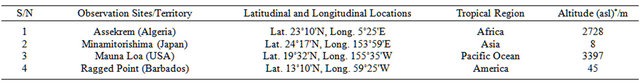
*asl = above sea level.
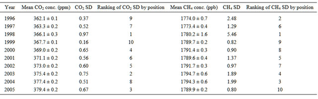
Table 2. Values of mean annual concentration of CO2 and CH4 with both the standard deviation and ranking for Assekrem station.
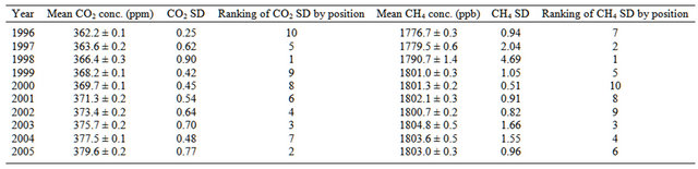
Table 3. Values of mean concentration of CO2 and CH4 with both the standard deviation and ranking for Minamitorishima station.
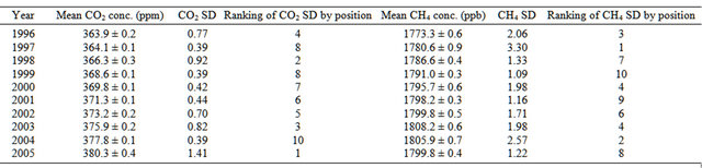
Table 4. Values of mean concentration of CO2 and CH4 with both the standard deviation and ranking for Mauna Loa station.
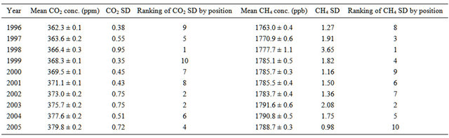
Table 5. Values of mean concentration of CO2 and CH4 with both the standard deviation and ranking for Ragged Point station.
greenhouse gas than similar increase in CO2. However, CH4 is less effective than CO2 on climate change because of its smaller atmospheric concentration.
The following are the summary of what was obtained for each of the observation sites considered.
3.1. Assekrem Station
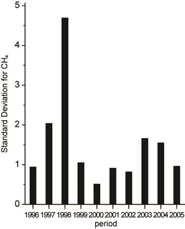
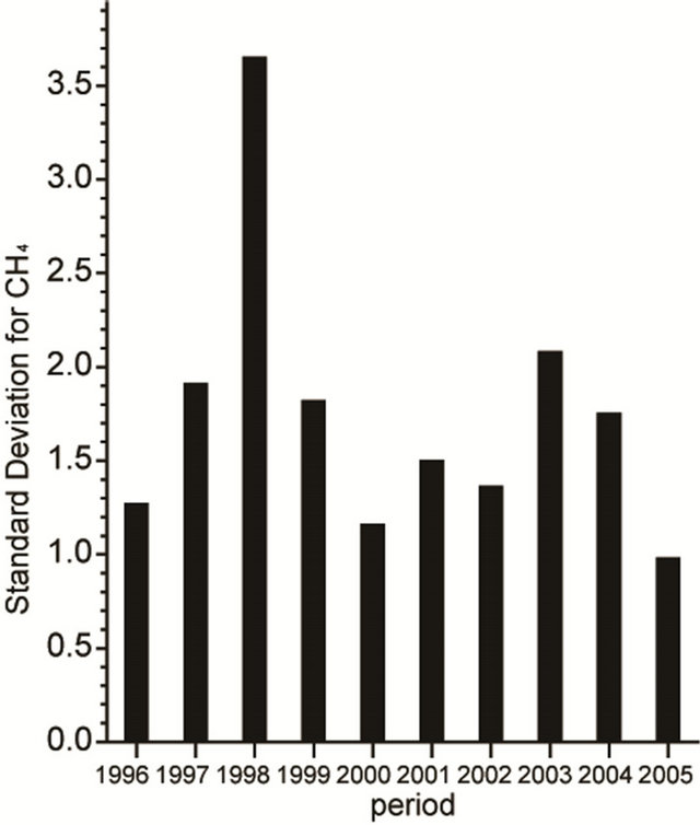
Table 2 shows the mean concentrations and SD for CO2 and CH4 gases. With reference to this table, the yearly variation shows that the SD which indicates warming has five of its highest values in terms of position ranking when arranged in decreasing order in 1998, 2005, 2003, 2002 and 1997 for CO2, while those of CH4 are 1998, 1997, 2003, 2004 and 1999 (Figures 1(a) and (b)). Thus, in this location, 1998 is the warmest year and coincides with the SD peak of CO2 and CH4.
3.2. Minamitorishima Station
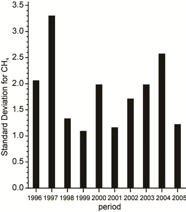
Table 3 shows the mean concentration and SD for these gases. With reference to this table the yearly variation shows that the SD has five of its highest values in terms of position ranking when arranged in decreasing order in 2005, 1998, 2003, 1996 and 2002 for CO2, while those for CH4 are 1997, 2004, 1996, 2003 and 2000 (Figures 2(a) and (b)). Thus, in this location 2005 and 1997 would be the warmest year in terms of both CO2 and CH4 respectively if these gases were the dominant factor of warming.
3.3. Mauna Loa Station
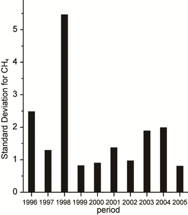
Table 4 shows the mean concentration and SD for these years. With reference to this table the yearly variation shows that the SD, has five of its highest values in terms of position ranking when arranged in decreasing order in 1998, 2002, 2003, 2005 and 1997 for CO2, while those for CH4 are 1998, 2003, 1997, 1999 and 2004 (Figures 3(a) and (b)). Thus, in this location 1998 is the warmest year and coincides with the SD peak of CO2 and CH4.
3.4. Ragged Point Station
Table 5 shows the mean concentration and SD for these gases. With reference to this table, the yearly variation shows that the SD which indicates warming has five of its highest values in terms of position ranking when arranged in decreasing order in 1998, 2003, 2005, 2000 and 2002 for CO2, while those for CH4 are 1998, 1996, 2004, 2003 and 2001 (Figures 4(a) and (b) ). Thus, in this location 1998 is the warmest year and coincides with
 (a)
(a)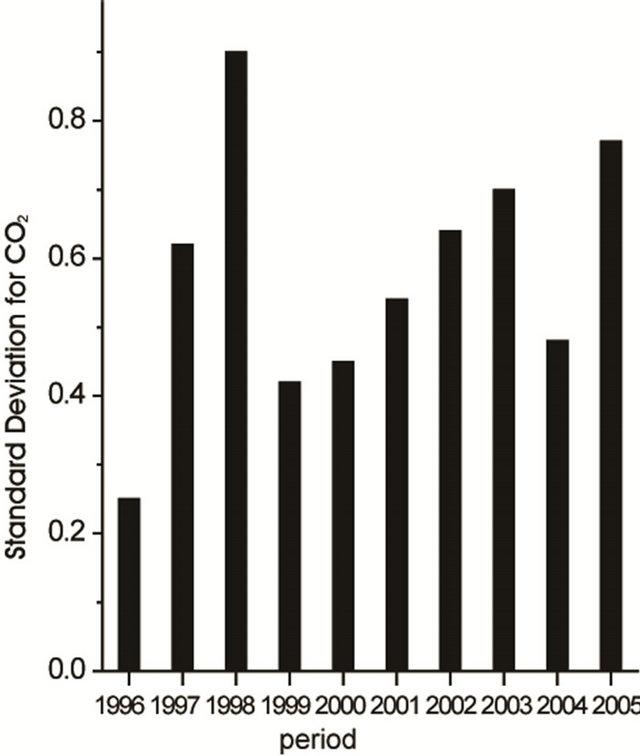 (b)
(b)
Figure 1. (a) and (b): Plot of annual standard deviation for CO2 and CH4 at Assekrem station.
 (a)
(a)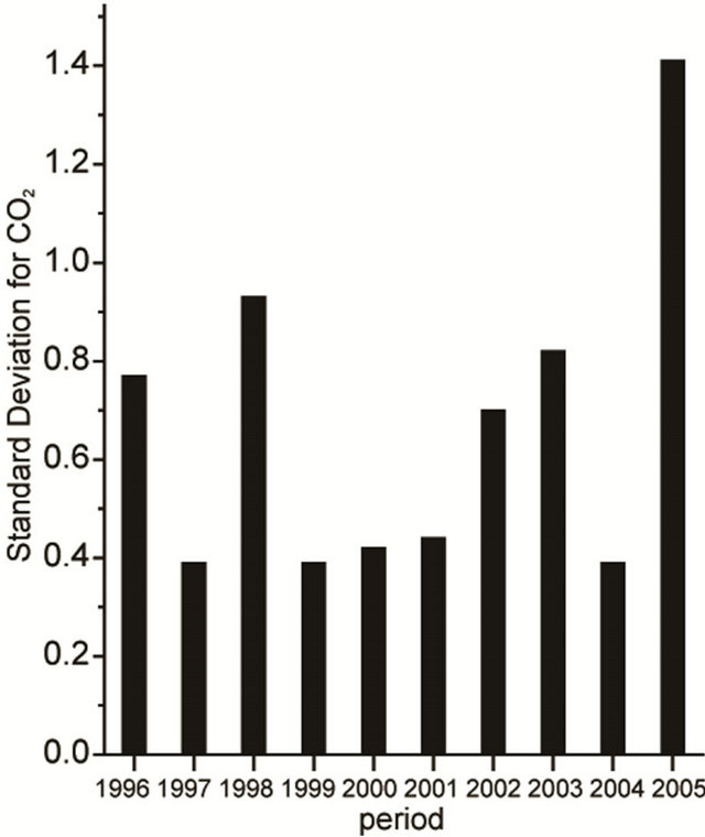 (b)
(b)
Figure 2. (a) and (b): Plot of annual standard deviation for CO2 and CH4 at Minamitorishima station.
 (a)
(a) (b)
(b)
Figure 3. (a) and (b): Plot of annual standard deviation for CO2 and CH4 at Mauna Loa station.
the SD peak of CO2 and CH4
4. Conclusion
The SD of the concentrations of CO2 and CH4 gases showed good correlations with the years associated with warming and serves as good climate proxies in a similar way to the traditionally used proxies of climate. Also, these standard deviations which indicate abnormality
 (a)
(a)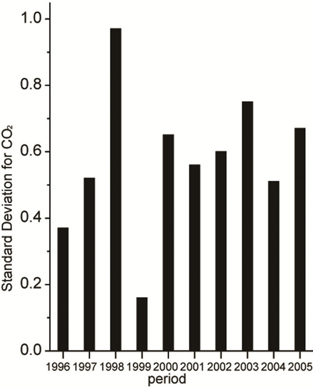 (b)
(b)
Figure 4. (a) and (b): Plot of annual standard deviation for CO2 and CH4 at Ragged Point station.
showed that 1998 is the warmest among the years considered for this study.
5. Acknowledgements
The authors wish to acknowledge the World Data Centre for Greenhouse Gases for making the data utilised in this work available.
REFERENCES
- T. Yeh and C. Fu, “Climatic Change—A Global Multidisciplinary Theme,” In: T. F. Malone and J. G. Roederer, Eds., ICSU: Global Change, Cambridge University Press, Cambridge, 1985, pp. 127-145.
- IPCC, “Scientific Assessment of Climate Change Intergovernmental Panel on Climate Change (IPCC) Report. WMO—UNEP,” Cambridge University Press, Cambridge, 1990.
- G. R. McGregor and S. Nieuwolt, “Tropical Climatology,” John Wiley and Sons, Hoboken, 1998.
- H. Le Treut, R. Somerville, U. Cubasch, Y. Ding, C. Mauritzen, A. Mokssit, T. Peterson and M. Prather, “Historical Overview of Climate Change,” In: S. Solomon, D. Qin, M. Manning, Z. Chen, M. Marquis, K. B. Avergt, M. Tiguor and H. L. Miller, Eds., Climate Change (2007): The Physical Basis. Contribution of Working Group 1 to the Fourth Assessment Report of the Intergovernmental Panel on Climate Change, Cambridge University Press, Cambridge and New York, 2007.
- National Oceanographic and Atmospheric Administration (NOAA) Paleoclimatology Program, “Introduction to Paleoclimatology,” 2002. http://www.ncdc.noaa.gov/paleo /paleo.proxy data.html
- A. Solow, and A. Huppert, “Optimal Multiproxy Reconstruction Reconstruction of Sea Surface Temperature from Corals,” Paleoceanography, Vol. 19, No. 4, 2004. doi:10.1029/2003PA000980
- K. L. De Long, T. M. Quinn and F. W. Taylor, “Reconstructing Twentieth-Century Sea Surface Temperature Variability in the South West Pacific: A Replication Study Using Multiple Coral Sr/Ca Records from New Caledonia,” Paleoceanography, Vol. 22, No. 4, 2007. doi:10.1029/2007PA001444
- Farlix Inc., “Anthropogenic Global Warming,” 2008. http://www.thefreedictionary.com/about.htm
- D. H. McIntosh and A. S. Thom, “Essentials of Meteorology,” Wykeham Publishing Ltd., London, 1973.
- O. E. Ogunsola and E. O. Oladiran, “Models of Greenhouse Gas Concentrations over Tropical Africa Using Auto-Regressive Moving Average Approach,” Journal of Science Research, Vol. 10, No. 1, 2011, pp. 80-89.
- D. R. Stang, “Trends in Atmospheric Methane,” Zipcodezoo.com the Bay Science Foundation Inc., 2009. http//zipcodezoo.com/
NOTES
*Corresponding author.