Journal of Sensor Technology
Vol.08 No.04(2018), Article ID:88820,8 pages
10.4236/jst.2018.84007
Recognition of Force Magnitude Applied to Pressure-Sensitive Conducting Rubber Sensors on the Basis of Frequency Table
Masato Ohmukai, Yasushi Kami
Department of Electrical and Computer Engineering, National Institute of Technology, Akashi College, Akashi, Japan

Copyright © 2018 by authors and Scientific Research Publishing Inc.
This work is licensed under the Creative Commons Attribution International License (CC BY 4.0).
http://creativecommons.org/licenses/by/4.0/


Received: October 14, 2018; Accepted: November 25, 2018; Published: November 28, 2018
ABSTRACT
This study aims to develop a force sensor system with a pressure-sensitive conductive rubber (PSCR), which shows the decrease of electrical resistance when pressure is applied. The biggest obstacle of the sensor is a poor reproducibility in the characteristic between the force and the resistance of the PSCR, which derived from a hysteresis and time variant properties. In this paper, we propose one method for recognizing a magnitude of the force to the PSCR using frequency tables. The validity of the proposed method is confirmed on the basis of experimental results.
Keywords:
Electric Conducting Rubber, Force Sensor, Frequency Table, Recognition of Force Magnitude

1. Introduction
Nowadays, force control has been more and more applied to a compliance control for robot arms as well as a feedback control of the humanoid robot hand for grasping fragile objects [1] [2] [3] [4] . The force control is actually realized by the feedback of the force detected by a force sensor [3] . Since the commercially available force sensor provides so small output signal as to require an amplifier, which results in high cost.
Pressure-sensitive electrically conductive rubber (PSCR) is one of the materials, the characteristics of which depend on the applied pressure. The PSCR consists of a rubber matrix where electrical conductive particles are scattered inside. When the pressure is applied, the particles are connected each other, then the electrical resistance decreases along with the pressure. The change in the resistance is detected as an electric voltage as described later. The PSCR is passive sensor so that it does not need a sophisticated amplifier. Since the PSCR is a soft rubber sheet, the form can be taken freely and it can be used even on a non-flat area. So the PSCR is so attractive for the cost effective force sensing that the application and improvement of the PSCR sensor have been performed recently [5] [6] [7] [8] .
Despite the advantages described above, the PSCR has the fault that it has a hysteresis property in the relationship between pressure and electrical resistance. Another serious problem is a poor reproducibility in measurement value. It really has made an obstacle for practical use. The idea in this article is that applied pressure is roughly recognized from the obtained time-series output data with the help of an experimentally prepared frequency table previously. The efficacy of this method is verified experimentally.
2. Experimental Details
2.1. Hardware of the Force Sensor
It should be described about the PSCR sensor. In the PSCR electrically conductive particles are randomly embedded in rubber matrix sheet as shown (left) in Figure 1. When pressure is applied on the sheet, the conductive particles are connected each other to form a current path as shown in the figure (right). This change can be detected as a decrease in electrical resistance.
There are two types of the PSCR depending on the materials of the conductive particles: metal or carbon. The scheme of the resistance variation is quite different in the two cases. The variation is shown in Figure 2. The left figure shows a step-like dependence and the right one shows a continuous variation. The latter analog-type PSCR is more suitable for the estimation of a pressure. We adopted this analog-type of PSCR sheet for the sensor.

Figure 1. A schematic diagram of a pressure-sensitive conductive rubber (left) and its state when the force is applied (right). Electric current can flow through the rubber by the application of force.
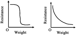
Figure 2. Two types of pressure-sensitive conduction rubber.
In our experiments, the PSCR (produced by PCR Technical) was cut in square of 4.4 cm. Two sheets of Al foil were attached to the both surfaces of the PSCR as the electrodes. This was sandwiched by two Al plates for the purpose that applied pressure should be uniform over the PSCR sensor even when weight was put on it locally.
The electric circuit for the detection is shown in Figure 3. The element of r in the figure indicates the sensor, where the resistance is varies with the applied force. The V in the left side is the applied voltage source (direct current) of 5.0 V. The R and C are a load resistor (3.9 kΩ) and a bypass capacitor (4.7 μF) for noise reduction, respectively. The Vo is the output voltage, which was transferred to a personal computer. The Vo is simply calculated by
To show the feature of the PSCR sensor briefly, the time responses (100-time repetition) of the output voltage Vo is shown in Figure 4 (100 times) when 4.9 N was applied at 0 s. The figure shows that it takes 0.4 s for the convergence. It is due to the inherent property of rubber. The figure also shows that the convergence value is dispersed so much. The relationship (10 times) between converged value of Vo and the applied force is shown in Figure 5. This figure also shows the dispersion of the converged values. The dynamic range lies around less than 150 N.

Figure 3. A detecting circuit for the rubber sensor r. Direct current voltage of 5 V was applied across the terminals (V in the figure), and the voltage of Vo was measured.

Figure 4. Time response of Vo with the applied force of 4.9 N (100 times).

Figure 5. The experimentally obtained Vo variations to the applied force (10 times).
2.2. Recognition of Pressure with a Frequency Table
We describe here the procedure of the recognition of pressure with a frequency table. At first, some variables are defined here. The origin of time is set to the time when the weight is put on the sensor. The passed time is defined to be ti (I = 1, 2, ∙∙∙, m), where each period is not necessary to be the same. The class of the observed voltage is labelled as j where the voltage is in the region between (j − 1)ΔVo and jΔVo. The weight to be distinguished is defined to be wk (k = 1, 2, ***, n). Frequency tables are prepared from the data obtained so many times with known weights in advance. The frequency table for the time ti is shown in Table 1. In this table p(i, j, k) is the number of times where the time is ti, the observed voltage is ranked at the label j, and the known weight of wk. The S(i, j) at the right ends of the table, represents the sum of all the number of times through all the known weight in the same voltage region.
Then the unknown weight is put on the sensor and the time response of the output voltage is measured. From the obtained time response, the weight can be estimated using the frequency table as follows. The output voltage at ti is in the weight range of ji, then the evaluation function of Jk for the weight wk is defined as
where ωi is the weight function. With the weight function, it can be opted which time should be emphasized for the evaluation. After the Jk for all k’s are calculated, the estimated weight of wz is obtained as
This method is very helpful for the case that the output voltage includes large experimental errors and that the weight is estimated roughly. The estimation is powerful especially when the measured weight is classified only to small number of discrete groups. However this can also be well applied to the case without large errors definitely.

Table 1. Frequency table for Vo(ti).
2.3. Recognition Trials
We describe here the conditions of the experiment for the recognition of the weight. We have chosen three kinds of force 4.9, 9.8 and 14.7 N that correspond to 0.5, 1.0 and 1.5 kgw, respectively. In this experiment ti is set to
And ΔVo was 0.025 V. the weight function was that ω1 and ω2 were 0.1, ω3 and ω4 were 0.2, ω5 and ω6 were 0.3 and ω7 was 0.4. The sampling period was 0.005 s. For the preparation of the frequency tables, the Vo response was measured 100 times for each weight. The duration of the measurement was 1 s.
3. Results of Recognition Rate Estimated by This Procedure
The time response of Vo was shown in Figure 4 when the force was 4.9 N. Similarly, those for 9.8 and 14.7 N were shown in Figure 6 and Figure 7, respectively. The static value of the output voltage at 1 s was centered at 0.2, 0.4 and 0.7 V, respectively. The observed surge under 0.1 V in Figure 7 derived from a transient experimental error. The average value and the range within the standard deviations of the response of Vo are shown in Figure 8 under 0.4 s. The range of the standard deviation is separated with each other perfectly at 0.4 s, although they are overlapped, as the time becomes smaller. So, it is rational that the weight function of ω is the larger for larger m. The frequency table at 0.4 s is shown in Table 2.
Using Table 2, the recognition tests were performed 100 times for each weight. The results are shown in Table 3. It shows that the weight of w1 is recognized w1 for 92% and w2 for 8%. There is no miss recognition between w1 and w3. All recognition rates are above 84%. This high recognition rate is surprising when it comes to a low-cost electric conducting rubber that has a hysteresis property.
This algorithm is shown to be able to evaluate the recognition rate for the discrete weight. This recognition algorithm can give a quantitative performance of the rubber force sensor. It is because the procedure is suitable for the time response output with large errors. This kind of system cannot be treated with any

Figure 6. Time response of Vo with the applied force of 9.8 N (100 times).

Figure 7. Time response of Vo with the applied force of 14.7 N (100 times).

Figure 8. The average and standard deviation of the response of each Vo(t) for three samples of w.
Table 2. Frequency table for a trial at i = 7 (t = 0.4).
Table 3. Results of the discrimination experiments.
sophisticated control theory anyway. This can be applied to other similar systems including large errors.
The next interesting point is that the recognition rate is studied among conducting rubber sensor under different situations. Further, the parameters such as ti and weight functions are needed to be adapted for the better recognition rate. In order to challenge a complicated system with random portion largely, this kind of primitive approach is inevitable even for further research.
4. Conclusion
The application of pressure-sensitive conductive rubber to a feedback system to measure the pressure is so cost effective but has a critical problem of its poor reproducibility. In the article, the method for recognition of applied force magnitude is proposed on the basis of frequency table. It was shown that the trial of this method gave the recognition rates above 84%. This method is decently effective for recognition of the data with large errors. We expect further investigations to verify the response when the load is removed as well as the dynamic identification of the load.
Acknowledgements
This work was partially supported by a Grant-in-Aid for Scientific Research No. 16K01430 from the Ministry of Education Science, Sports, and Culture, for which the authors are grateful.
Conflicts of Interest
The authors declare no conflicts of interest regarding the publication of this paper.
Cite this paper
Ohmukai, M. and Kami, Y. (2018) Recognition of Force Magnitude Applied to Pressure-Sensitive Conducting Rubber Sensors on the Basis of Frequency Table. Journal of Sensor Technology, 8, 88-95. https://doi.org/10.4236/jst.2018.84007
References
- 1. Lee, M.H. and Nicholls, H.R. (1999) Review Article Tactile Sensing for Mechatronics—A State of the Art Survey. Mechatronics, 9, 1-31. https://doi.org/10.1016/S0957-4158(98)00045-2
- 2. Li, A., Hsu, P. and Sastry, S. (1989) Grasping and Coordinated Manipulation by a Multifingered Robot Hand. International Journal of Robotics Research, 8, 33-50. https://doi.org/10.1177/027836498900800402
- 3. Berger, A.D. and Khosla, P.K. (1991) Using Tactile Data for Real-Time Feedback. International Journal of Robotics Research, 10, 88-102. https://doi.org/10.1177/027836499101000202
- 4. Schmidt, P.A., Mael, E. and Wurtz, R.P. (2006) A Sensor for Dynamic Tactile Information with Applications in Human-Robot Interaction & Object Exploration. Robotics and Autonomous Systems, 54, 1005-1014. https://doi.org/10.1016/j.robot.2006.05.013
- 5. Ohmukai, M., Kami, Y. and Matsuura, R. (2012) Electrode for Force Sensor of Conductive Rubber. Journal of Sensor Technology, 2, 127-131. https://doi.org/10.4236/jst.2012.23018
- 6. Ohmukai, M., Kami, Y. and Ashida, K. (2013) Conducting Rubber Force Sensor: Transient Characteristics and Radiation Heating Effect. Journal of Sensor Technology, 3, 36-41. https://doi.org/10.4236/jst.2013.33007
- 7. Ohmukai, M. and Kami, Y. (2016) A Sputtering Deposition of Al Enhances the Output Reproducibility in a Conducting Rubber Force Sensor. Journal of Sensor Technology, 6, 46-55. https://doi.org/10.4236/jst.2016.63004
- 8. Ohmukai, M., Kami, Y. and Yawata, R. (2016) Stacked Structure Improves Output Reproducibility of Rubber Force Sensor. Journal of Sensor Technology, 6, 75-80. https://doi.org/10.4236/jst.2016.63006