Journal of Sensor Technology
Vol.1 No.3(2011), Article ID:7654,4 pages DOI:10.4236/jst.2011.13009
Non-Contact Stress Measurement during Tensile Testing Using an Emat for SH0-Plate Wave and Lamb Wave
Department of Intelligent Mechanical Engineering, Faculty of Engineering, Fukuoka Institute of Technology, Fukuoka, Japan
E-mail: murayama@fit.ac.jp
Received July 8, 2011; revised August 14, 2011; accepted August 24, 2011
Keywords: Nondestructive Inspection, Ultrasonic Sensor, Stress, Acoustoelasticity, SH0-Plate Wave, S0-Lamb Wave, Tensile Test, Electromagnetic Acoustic Transducer
Abstract
The stress on a test specimen during tensile testing is generally measured by a strain gauge. This method has some problems in that it would influence the measurement conditions of the tensile test and can evaluate only the position at which the strain gauge is attached. The acoustoelastic method is proposed as a method replacing the strain gauge method. However, an ultrasonic sensor with a piezoelectric oscillator requires a coupling medium to inject an ultrasonic wave into a solid material. This condition, due to the error factor of the stress measurement, makes it difficult for the ultrasonic sensor to move on the specimen. We then tried to develop a non-contact stress measurement system during tensile testing using an electromagnetic acoustic transducer (EMAT) with an SH0-plate wave and S0-Lamb wave. The EMAT can measure the propagation time in which the ultrasonic wave travels between a receiver and a transmitter without a coupling medium during the tensile testing and can move easily. The interval between the transmitter and the receiver is 10mm and can be moved along the parallel direction or the vertical direction of the tensile load. The transit time was measured by a cross-correlation method and converted into the stress on the test specimen using the acoustoelastic method. We confirmed that the stress measurement using an SH0-plate wave was superior to that with an S0-Lamb wave.
1. Introduction
A strain gauge is widely used as a stress measurement method, but it can only measure stress on the specimen only at the position where it would be attached. It may then be possible to supplement a strain gauge, if we could develop a measurement system that evaluates stress on a test specimen at an arbitrary position while loaded by a tensile machine. There is a stress measurement method that uses an ultrasonic wave as one of the methods considered [1-4]. However, it was necessary for a commercial ultrasonic wave transducer to touch the solid material through a coupling medium such as oil or water to allow the ultrasonic wave to penetrate the material [5]. It was difficult to do a high-speed and accurate evaluation that did not influence the material during the mechanical test. Therefore, we have developed a system that can evaluate stress distribution in a tensile specimen during a tensile test using an electromagnetic acoustic transducer (EMAT) which does not need a coupling medium [6-8].
2. Principle of Stress Measurement
Generally, the transit time of an ultrasonic wave which travels a fixed distance is obtained by dividing the propagation distance by the ultrasonic wave velocity. However, when a compressive or tensile stress is applied to the material, the ultrasonic velocity slightly changes in proportion to the load stress the propagation time will also change. This is generally called the acoustoelastic law [1-4]. Therefore, the load stress can be evaluated from the transit time change as shown in Equation (1). However, when carrying out a nondestructive evaluation using a contact type ultrasonic transducer, the sensor needs to be in contact with the measurement specimen through a coupling medium as shown in Figure 1(a). Because the velocity change based on the acoustoelastic
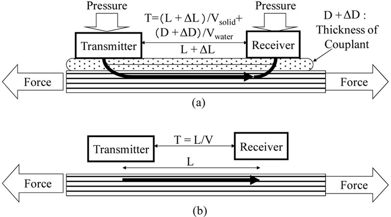
Figure 1. Problem and solution for stress measurement evaluation by acoustoelastic method; (a) Problem with a contact-type ultrasonic probe; (b) Improvement using a non-contact type ultrasonic probe.
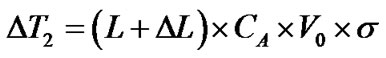
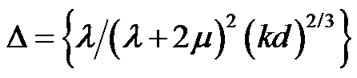
law is very minute, the thickness change in a coupling medium and the distance change between the transmitter and the receiver fixed to the specimen will influence the transit time measurement by an error factor as shown in Equation (3). Moreover, a conventional ultrasonic sensor directly influences the mechanical test results, because it would load the test specimen itself. We thought that a non-contact sensor can solve these problems as shown in Figure 1(b) and that Equation 2 could be used to evaluate the tensile stress.
 (1)
(1)
 (2)
(2)
 (3)
(3)
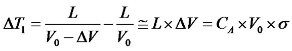
L: Distance between the transmitter and the receiver
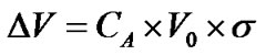
ΔL: Elongation of L V0: Velocity without any stress in the specimen
ΔV: Velocity change due to the stress
σ: Stress E: Youngs elastic constant CA: Acoustoelastic constant
ΔT1: Transit time change due to the stress
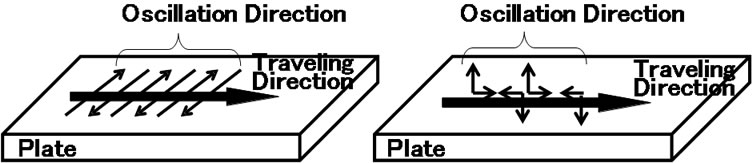
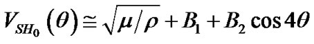
ΔT2: Transit time change due to the stress and the traveling distance change We decided to use a plate wave that can cause the displacement direction of an ultrasonic wave to become paralleled relatively to the tensile direction of the tensile machine, though there are several kinds of ultrasonic wave modes. We especially used the fundamental mode of a shear horizontal plate wave (SH0-plate wave) as shown in Figure 2(a) because it did not have a velocity distribution for a plate thickness change as shown in Equation (4) [11,12]. We then used an S0-Lamb wave as shown in Figure 2(b) which has a velocity dispersion relative to the change in the plate thickness for comparing the evaluation ability as shown in Equation(5) [11,12].
 (a) (b)
Figure 2. (a) Displacement pattern of a Lamb wave and an SH-plate wave. (a) SH-plate wave; (b) Lamb wave.
 (4)
(4)
 (5)
(5)
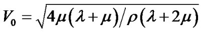
ρ: density
λ and μ: Lame constant
θ: Traveling angle relative to the rolling direction A1, A2, A3, B1, B2: Constant by computing using elastic constants
3. Basic Structure of an Ultrasonic Sensor [6-8]
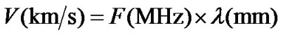
The basic structure of a trial transducer is shown in Figure 3. It consists of an electromagnet and a pair of meander line sensor coils of which one is the transmitter and the other is the receiver. Although there is a Lorenz force and a magnetostrictive effect for the drive force of an electromagnetic acoustic transducer (EMAT), we developed a magnetostrictive type EMAT. A static magnetic field is applied to the specimen and arranged to become the greatest change in the magnetostriction when the magnetic field changes. When a periodic dynamic magnetic field is then superimposed on an optimum static magnetic field, the greatest change in the magnetostriction can be induced in the material. When the intervals between the electrodes of the sensor coil are coincident with the wavelength of the plate wave, this is converted into the plate wave. The velocity of the plate wave is calculated by multiplying the drive frequency and the wavelength. The driving force uses a highfrequency magnetostrictive vibration generated in the direction of the compound’s magnetic field by combining the dynamic magnetic field generated by a high-frequency electric current in the sensor coil and the static field due to the electromagnet. This could generate an S0-Lamb wave when the electromagnet was set up parallel to the sensor coil pair and could generate an SH0-plate wave when the electromagnet was set up vertical to the sensor coil pair. The distance between the electric fingers (W) was determined to be the half-wavelength computed using Ex. (6). Therefore, the distance between the electric
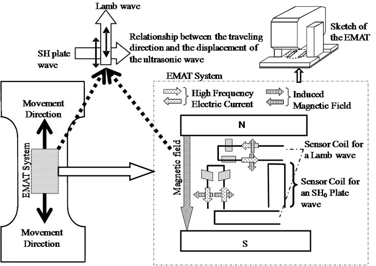
Figure 3. Basic principle of an electromagnetic acoustic transducer for an SH0-plate wave and an S0-Lamb wave.
fingers was 2.6 mm for the S0-mode Lamb wave and 1.5 mm for the SH0-plate wave using a thin (0.5 mm) steel sheet, because a thin steel sheet of 0.5 mm thickness was used as the material for the test piece. The distance between the transmitter and receivers was typically 10 mm. The transmitted signal to drive the transmitter is a four-cycle burst-type pulse with a drive frequency of 2 MHz, and the maximum voltage was 1000 V. The impedance of the transmitter at the 2 MHz drive frequency was 4.3 Ω on the test piece, and the number of turns of the sensor coil was five. The amplifier is able to amplify the signal in the frequency range from 2 kHz to 4 MHz with an amplification magnitude of 40 dB. The impedance of the receiver at the 2 MHz drive frequency was 22.3 Ω on the test piece, and the number of turns of the sensor coil was ten. The applied voltage from the power supply to drive the electromagnet was 40 V, and the resistance of the magnetic coil in the electromagnet was 4 Ω. The number of turns of the magnetic coil was 700.
 (6)
(6)
4. Stress Evaluation System
An outline of the trial measurement system is shown in Figure 4. The system is composed of a portable type tensile machine, the tensile specimen and a sensor mounting system. The tensile machine can tensile the specimen with a maximum load of 10 kN. The tensile specimen has a 0.25 mm thickness, a 200 mm maximum length and a 25 mm width. As shown in Figure 4, a direct ultrasonic wave arriving from the transmitter to the receiver was observed.
Both sensors can also move over the tensile specimen in the tensile direction. The speed was 1 mm/sec, and the sensors can be accurately returned to the same position by computer control.
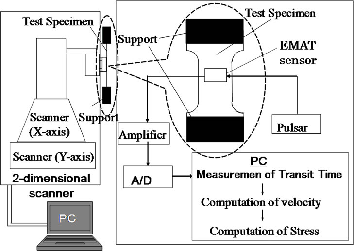
Figure 4. Evaluation system for stress in a tensile specimen while loading.
5. Measurement Method of Transit Time
We used an SH0-plate wave and an S0-Lamb wave to evaluate the average tensile stress over the entire thickness and a distance of 10 mm in the tensile direction. Therefore, the transit time can be estimated to be about 2 μs - 3 μs, if we assume the ultrasonic velocity to be 3,200 m/s or 5.900 m/s. Also, if we assume an acoustic elasticity coefficient of 10–5/MPa, the change in the transit time due to the stress can be estimated to be 0.2 ns - 0.3 ns for each 10 MPa. The following transit time method was then executed as an evaluation method with high measurement accuracy. The transit time of the same position was measured to consider the initial anisotropy of the material before it was loaded. Next, the transit time was measured after loading. Finally, the difference between both transit times was calculated. This method also has the effect of removing the influence of the temperature of the test piece. Moreover, even when the sheet thickness of the test pieces is different, this influence can be removed by considering the difference as shown in Figure 5. The cross correlation coefficient (Gxy) of the received signal both before and after loading was calculated by delaying the start time of the received signal at the same measuring position as shown in Equation (7) [13,14].
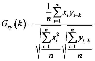 (7)
(7)
Σxi: Discrete received signal before loading
Σyi: Discrete received signal after loading n: The number of discrete received signal data points k: Corresponding to the delay time ( )
)
Δt: Interval between the time resolution
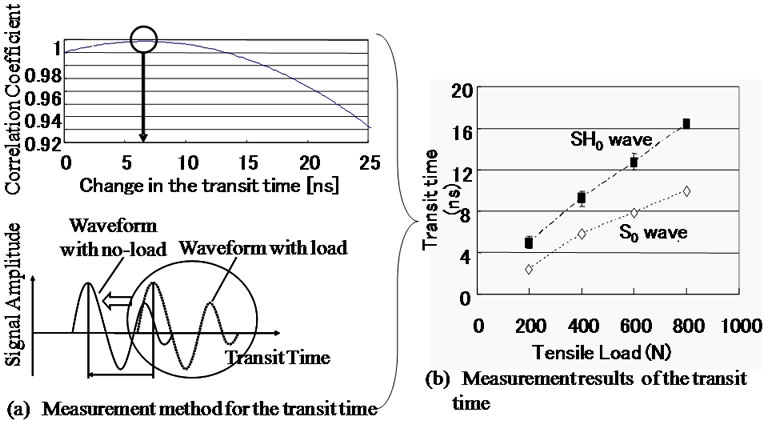
Figure 5. Precise transit time measuring method and the measured transit time.
Figure 5(b) shows the relationship between the tensile stress and the change in the transit time. The change ratios of the transit time of the SH0-mode and the S0-mode were (0.012 ± 0.000085) ns/MPa and (0.019 ± 0.00016) ns/MPa by using the least squares method. These values became –7.08 ± 0.05 × 10⁻⁶ (1/MPa) in case of SH0- mode and –6.08 ± 0.05×10⁻⁶ (1/MPa) in case of S0-mode when converting them into the acoustoelastic coefficients.
6. Test Specimen
The test piece shown in Figure 6 was fabricated to evaluate the anti-symmetric stress distribution in the center of the test piece. The total length was 200 mm, the width of the center was 120 mm and the thickness was 0.25 mm. The stress values described at positions A-K in the figure were calculated by dividing the tensile force by the cross section.
7. Experimental Results
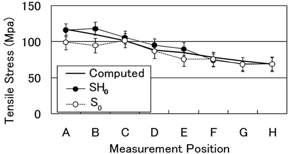
Figure 7(a) shows the measured stress distribution in the tensile specimen at a tensile force of 350 N, while the sensor was moving along the tensile direction. The difference between the evaluated value using an SH0-plate wave and the calculated value was +3.3 MPa on the average, and the error at any position of the test specimen was almost the same value. Next, the difference between the evaluated value using an S0-Lamb wave and the calculated value was –6.3 MPa on the average; especially, the error at the A and B positions on the test specimen was about –16.0 MPa.
Figure 7(b) shows the measured stress distribution in the tensile specimen at a tensile force of 700 N, while the sensor was moving along the tensile direction. The difference between the evaluated value using an SH0-plate wave and the calculated value was –2.4 MPa on the average, and the error at any position of the test specimen was almost the same value. Next, the difference between
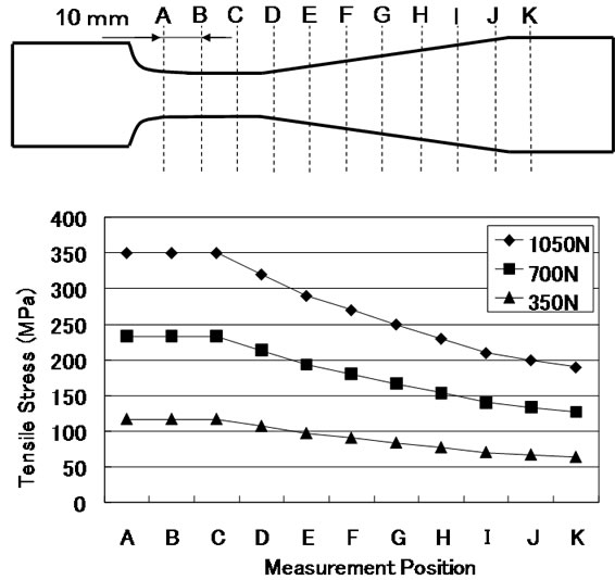
Figure 6. The computed stress value on a trial tensile specimen at a fixed tensile force.
the evaluated value using an S0-Lamb wave and the calculated value was –18.0 MPa on the average, especially, the error at the A and B positions on the test specimen was about –40 MPa.
Figure 7(c) shows the measured stress distribution in the tensile specimen at a tensile force of 1050 N, while
 (a)
(a)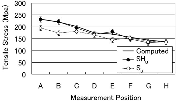 (b)
(b)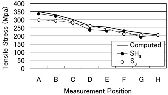 (c)
(c)
Figure 7. Measured and computed stress value. (a) 350 N; (b) 700 N; (c) 1050 N.
the sensor was moving along the tensile direction. The difference between the evaluated value using an SH0- plate wave and the calculated value was –10 MPa on the average, and the error at any position of the test specimen was almost the same value. Next, the difference between the evaluated value using an S0-Lamb wave and the calculated value was –14 MPa on the average; especially, the error at the A and B positions on the test specimen was about –34 MPa.
8. Influence of a Plate Thickness Change
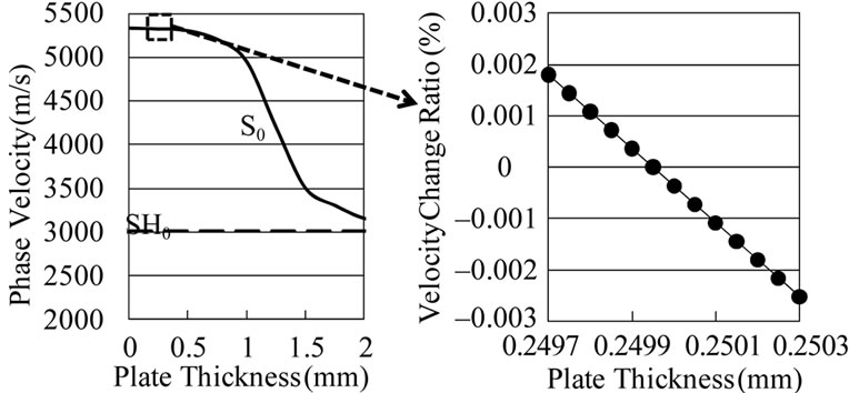
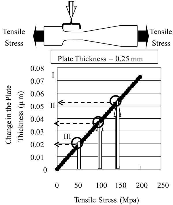
It was checked why the evaluation results at position A and B using an S0-Lamb wave were underestimated compared to the computation results. At first, the change in the velocity of an S0-Lamb wave was evaluated when the tensile specimen was pulled. The dependence of the S0-Lamb wave velocity on the thickness change was calculated using Equation (5). Figure 8 shows the calculation results, which indicate that the velocity change in an S0-Lamb wave becomes 0.00135% if the sheet thickness change is 0.1 μm. Next, the sheet thickness change from Equation (8) was computed when the test specimen was pulled by the tensile machine. The results are shown in Figure 9(a). The value of the vertical axis shows the change in the plate thickness at the minimum width part (A) of the test specimen. Figure 9(b) shows the change in the velocity of the S0-Lamb wave and the stress evaluation error due to the change in the test specimen. Black square marks in Figure 9(b) show the velocity change in an S0-Lamb wave due to the sheet thickness change calculated from the results of Figure 9(a) using Figure 8(b). The error value in the evaluated stress value due to the change in the S0-Lamb wave velocity is shown by white square marks in Figure 9(b).
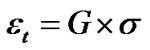 (8)
(8)
εt: strain, G: vertical elastic constant, σ: stress
Figure 10 shows the relationship between the maximum tensile stress on the tensile specimen for the tensile force and the error in the estimated stress value at position A, the error value in the stress computed from Figure 10(b). It is shown that the stress evaluation using an S0-Lamb wave contained an evaluation error of more than 10MPa because in the plate thickness change of the test specimen under the measurement conditions.
Figure 11 shows the experimental result using another shape of test specimen (B), which is expected to have the same tensile stress in its center area. The evaluation results using an SH0-plate wave agreed well with the computed value within an accuracy of 10 MPa tensile stress.
 (a) (b)
Figure 8. Plate thickness and the change in the velocity. (a) Velocity dependence due to the change in the plate thickness. (b) Velocity change ratio of an S0-Lamb wave due to the change in the plate thickness.
 (a)
(a)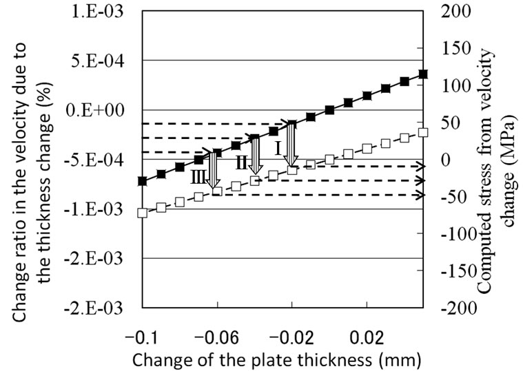 (b)
(b)
Figure 9. Velocity change and compensated stress value for a plate thickness change. (a) Change in the plate thickness due to the tensile stress at A-B on the tensile specimen; (b) Change in the S0-Lamb wave velocity and the evaluation error in the stress due to the change in the plate thickness.
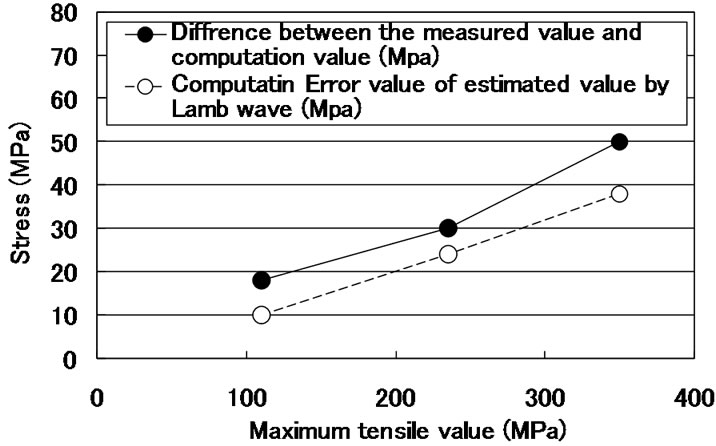
Figure 10. Stress evaluation results using tensile specimen A.
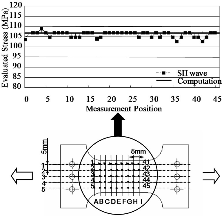
Figure 11. Stress evaluation results using tensile specimen B.
9. Conclusions
A stress evaluation system using an EMAT with an SH0-plate wave was developed during tensile testing. The system could fundamentally evaluate the average stress along the tensile direction in the tensile specimen of 0.25 mm thickness with 10 MPa accuracy while moving. We could also confirm that the measurement system using the SH0-plate wave was superior to that with an S0-lamb wave. The reproducibility of the measurement results was also excellent.
We will develop an EMAT with an SH-surface wave to be applicable for a test specimen with greater plate thickness.
10. References
[1] D. I. Crecraft, “The Measurement of Applied and Residual Stress in Metals Using Ultrasonic Waves,” Journal of Sound and Vibration, Vol. 5, No. 1, 1967, pp. 173-192. doi:10.1016/0022-460X(67)90186-1
[2] K. Okada, “Stress-Acoustic Relation for Stress Measurement by Ultrasonic Techniques,” Journal of the Acoustical Society of Japan (E), Vol. 1, 1980, pp. 193-200.
[3] Y. H. Pao, W. Sache and H. Fukuoka, “Acoustoelasticity and Ultrasonic Measurement of Residual Stress,” Physical Acoustics, Vol. 15, 1984, pp. 61-143.
[4] M. Hirao, H. Fukuoka, H. Toda, Y. Sotani and S. Suzuki, “Non-Destructive Evaluation of Hardening Depth using Surface-Wave Dispersion Patterns,” Journal of Mechanical Working Technology, Vol. 8, No. 2-3, 1983, pp. 171-179. doi:10.1016/0378-3804(83)90035-9
[5] B. Raj, V. Rajendran and P. Palanichamy, “Ultrasonic Transducers,” Science and Technology of Ultrasonics, Alpha Science International Ltd., Oxford, 2004, pp. 37-67.
[6] R. B. Thompson, “A Model for the Electromagnetic Generation and Detection of Rayleigh and Lamb Wave,” IEEE Transactions on Sonics and Ultrasonics, Vol. 20, 1973, pp. 340-346.
[7] M. Hirao and H. Ogi, “Development of EMAT Techniques,” EMATS for Science and Industry, Kluwer Academic Publishers, London, 2003, pp. 13-82.
[8] G. Alers and H. Ogi, “Handbook of Elastic Properties of Solids, Liquids and Gases,” In: M. Levy, H. Bass, R. Stern and V. Keppens, Eds., EMAT Techniques, Academic Press, New York, 2001, pp. 263-281.
[9] H. Ogi, E. Goda and M. Hirao, “Increase of Efficiency of Magnetostriction SH-Wave EMAT by Angled Bias Field,” Japanese Journal of Applied Physics, Vol. 42, 2003, pp. 3020-3024. doi:10.1143/JJAP.42.3020
[10] M. Hirao, H. Ogi and H. Yasui, “Contactless Measurement of Bolt Axial Stress Using a Shear-Wave Electromagnetic Acoustic Transducer,” NDT & E International, Vol. 34, No. 3, 2001, pp. 179-183. doi:10.1016/S0963-8695(00)00055-4
[11] M. Hirao and H. Ogi, “On-line Texture Monitoring on Steel Sheets,” EMATS for Science and Industry, Kluwer Academic Publishers, London, 2003, pp. 197-213.
[12] M. Hirao and H. Fukuoka, “Dispersion Relation of Plate Modes in Anisotropic Polycrystalline Sheets,” Journal of the Acoustical Society of America, Vol. 85, No. 6, 1989, pp. 2311-2315. doi:10.1121/1.397777
[13] E. P. Papadakis, “Ultrasonic Pulse Velocity by the Pulse-Echo-Overlap Method Incorporating Diffraction Phase Correlation,” Journal of the Acoustical Society of America, Vol. 42, 1967, pp. 1045-1051.
[14] H. J. McSkimin, “Pulse Superposition Method for Measuring Ultrasonic Wave Velocities in Solids,” Journal of the Acoustical Society of America, Vol. 33, No. 1, 1961, pp. 12-16. doi:10.1121/1.1908386