Journal of Signal and Information Processing
Vol.07 No.01(2016), Article ID:63579,11 pages
10.4236/jsip.2016.71002
Convergence Curve for Non-Blind Adaptive Equalizers
Monika Pinchas
Department of Electrical and Electronic Engineering, Ariel University, Ariel, Israel

Copyright © 2016 by author and Scientific Research Publishing Inc.
This work is licensed under the Creative Commons Attribution International License (CC BY).
http://creativecommons.org/licenses/by/4.0/


Received 2 November 2015; accepted 16 February 2016; published 19 February 2016
ABSTRACT
In this paper a closed-form approximated expression is proposed for the Intersymbol Interference (ISI) as a function of time valid during the entire stages of the non-blind adaptive deconvolution process and is suitable for the noisy, real and two independent quadrature carrier input case. The obtained expression is applicable for type of channels where the resulting ISI as a function of time can be described with an exponential model having a single time constant. Based on this new expression for the ISI as a function of time, the convergence time (or number of iteration number required for convergence) of the non-blind adaptive equalizer can be calculated. Up to now, the equalizer’s performance (convergence time and ISI as a function of time) could be obtained only via simulation when the channel coefficients were known. The new proposed expression for the ISI as a function of time is based on the knowledge of the initial ISI and channel power (which is measurable) and eliminates the need to carry out any more the above mentioned simulation. Simulation results indicate a high correlation between the simulated and calculated ISI (based on our proposed expression for the ISI as a function of time) during the whole deconvolution process for the high as well as for the low signal to noise ratio (SNR) condition.
Keywords:
Non-Blind Adaptive Equalizers, Non-Blind Adaptive Deconvolution, Acquisition Time, Convergence Time

1. Introduction
We consider a non-blind deconvolution problem in which we observe the output of an unknown, possibly nonminimum phase, linear system (single-input-single-output (SISO) finite impulse response (FIR) system) from which we want to recover its input (source) using an adjustable linear filter (equalizer) and training symbols [1] . During transmission, a source signal undergoes a convolutive distortion between its symbols and the channel impulse response. This distortion is referred to as ISI [1] -[3] . It is well known that ISI is a limiting factor in many communication environments where it causes an irreducible degradation of the bit error rate thus imposing an upper limit on the data symbol rate [1] . In order to overcome the ISI problem, an equalizer is implemented in those systems [1] [4] -[7] . The equalization performance in the residual ISI point of view depends on the channel characteristics, on the added noise, on the step-size parameter used in the adaptation process, on the equalizer’s tap length and on the input signal statistics [1] . Fast convergence speed and reaching a residual ISI where the eye diagram is considered to be open are the main requirements from a blind and non-blind equalizer [1] . According to [1] , fast convergence speed may be obtained by increasing the step-size parameter. But increasing the step-size parameter will lead to a higher residual ISI which might cause the recovery process of the sent symbols more difficult and maybe even impossible. Up to now, there is no closed- form expression for the ISI as a function of time for the non-blind adaptive case, nor a closed-form expression for the convergence time (or number of iteration required for convergence) even when all the channel coefficients are known. Therefore, the system designer had to carry out many simulations in order to figure out the desired step-size parameter and equalizer’s tap length for a required convergence speed and residual ISI.
In this paper, we propose for the real and two independent quadrature carrier input case, a closed-form approximated expression for the ISI as a function of time (or number of iteration number) valid during the entire stages of the iterative deconvolution process. This new expression depends on the SNR, on the step-size parameter used in the adaptation process, on the equalizer’s tap length, on the input signal statistics and on the channel’s power (which is measurable). The obtained expression is applicable for type of channels where the resulting ISI as a function of time can be described with an exponential model having a single time constant. Based on this new expression for the ISI as a function of time (or number of iteration number), the convergence time (or number of iteration number required for convergence) of the non-blind adaptive equalizer is obtained.
The paper is organized as follows: After having described the system under consideration in Section 2, the closed-form approximated expression for the ISI as a function of time (or number of iteration number) is introduced in Section 3. In Section 4 simulation results are presented and the conclusion is given in Section 5.
2. System Description
The system under consideration is illustrated in Figure 1, where we make the following assumptions:
1) The input sequence  belongs to a two independent quadrature carrier case constellation input with variance
  where
where  and
and  are the real and imaginary parts of
  respectively.
2) The unknown channel  is a possibly nonminimum phase linear time-invariant filter in which the transfer function has no “deep zeros”, namely, the zeros lie sufficiently far from the unit circle.
3) The equalizer  is a tap-delay line.
4) The noise  is an additive Gaussian white noise with zero mean and variance
  where
where  is the expectation operator.
The sequence  is transmitted through the channel
  and is corrupted with noise
 . Therefore, the equalizer’s input sequence
  may be written as:
 (1)
(1)
where “ ” denotes the convolution operation. The equalized output sequence is defined by:

Figure 1. Block diagram of a baseband communication system.
 (2)
(2)
where  is the convolutional noise (convolutional error) due to non-ideal equalizer’s coefficients (
 ) and
) and . Next we turn to the adaptation mechanism of the equalizer which is based on training symbols [1] [4] -[8] :
 (3)
(3)
where  is the step-size parameter,
  is the equalizer vector where the input vector is
 and N is the equalizer's tap length. The operator
  denotes for transpose of
the function  and the operator
  denotes for the conjugate operation of
 . Please note that for the non-blind adaptive case, during the training period a known data sequence is transmitted. A replica of this sequence is made available at the receiver in proper synchronism with the transmitter, thereby making it possible for adjustments to be made to the equalizer coefficients in accordance with the adaptive filtering algorithm employed in the equalizer design [1] [8] .
3. ISI as a Function of Time
In this section we derive a closed-form approximated expression for the ISI a function of time or as a function of number of iteration number. Based on this expression, a closed-form approximated expression is obtained for the convergence time (or number of iteration number required for convergence) of the non-blind adaptive equalizer. Since we deal with the real and two independent quadrature carrier case, we start our derivations first with the real valued case and then turn to the two independent quadrature carrier one.
Theorem 1. For the following (additional) assumptions:
1) The convolutional noise , is a zero mean, white Gaussian process with variance
 .
.  and
and  are the real and imaginary parts of
  and
and .
.
2) The variance of the source signal  as well as its higher moments are known.
 .
.
3) The convolutional noise  and the source signal are independent. Thus,

The ISI as a function of the discrete time is approximately expressed as:
 (4)
(4)
where  is the largest integer not greater than Q and
  is the sampling time.
Comments:
Assumptions 1 and 3 were also made in [9] -[11] and in [12] . As already was noted in [13] and [14] , the described model for the convolutional noise  is applicable during the latter stages of the process where the process is close to optimality [12] . According to [12] , in the early stages of the iterative deconvolution process, the ISI is typically large with the result that the data sequence and the convolutional noise are strongly correlated and the convolutional noise sequence is more uniform than Gaussian [15] . However, satisfying equalization performance were obtained by [11] and others [13] in spite of the fact that the described model for the convolutional noise
  was used. These results ( [11] [13] ) may indicate that the described model for the convolutional noise
  can be used (maybe not in the optimum way) also in the early stages where the “eye diagram” is still closed. Concerning assumption 2, since we deal with the non-blind case, all the higher moments of the source input are known at the receiver.
Proof. Recently [1] , an expression for  was derived for the non-blind adaptive case:
 (5)
(5)
which was based on [14] where both sides of (3) were multiplied with the row vector
 and the expression of
  was
was
used where  and
and . Please note that
 (6)
(6)
Now, we divide both sides of (5) with  and obtain:
 (7)
(7)
with
 (8)
(8)
where  was approximated with
  as was done in [1] and [14] and
 . The expression in (7)
can be approximately seen as a first order differential equation with the following solution for :
:
 (9)
(9)
where  is a constant value obtained via the ISI at time zero as will be explained in the following. Based on [14] , the relationship between the ISI and the convolutional noise power for the real or two independent carrier case is expressed as:
 (10)
(10)
Thus, by dividing both sides of (9) with  we obtain based on (10):
 (11)
(11)
Next, we find a closed-form expression for  via (11) at time
 :
:
 (12)
(12)
In order to complete our proof, we use the relation of  in (11) and keep in
mind that we have to wait until the whole convolution process is finished in (6) to create  in order to use it
in (7). Thus, we substitute  in the exponent of (11) in order to get the ISI as a function of the
discrete time which completes our proof.
Based on (4), the number of iteration number required for convergence can be obtained:
 (13)
(13)
where  is the reached ISI level after n iterations.
4. Simulation
In this section we test our new proposed expression for the ISI as a function of time (4) via simulation. For this purpose we use two different constellation inputs:
A 16QAM input case (a modulation using ±{1,3} levels for in-phase and quadrature components) and the QPSK input case (a modulation using ±{1} levels for in-phase and quadrature components). The following six channels were considered:
Channel1 (initial ): The channel parameters were determined according to [11] :

Channel2 (initial ): The channel parameters were determined according to:

Channel3 (initial ): The channel parameters were determined according to:

Channel4 (initial ): The channel parameters were determined according to:

Channel5 (initial ): The channel parameters were determined according to [16] :
 .
.
Channel6 (initial ): The channel parameters were determined according to:
 .
.
The equalizer was initialized by setting the center tap equal to one and all others to zero.
Please note that according to [11] , Channel1 is a telephone channel. In addition, Channel2-Channel4 are variations of Channel1 in order to get different values for the initial ISI. In the following we denote the ISI as a function of time (4) as the “Calculated ISI” and the “Simulated ISI” as the ISI as a function of time obtained via the simulation. Figures 2-13 show the ISI as a function of the iteration number (time) calculated according to (4) compared with the simulated results for six different channels, two different input constellations, various equalizer’s tap-length, various values for the SNR and step-size parameter. According to Figures 2-13, a high correlation is observed between the simulated and calculated (according to (4)) results. It should be pointed out that there might be cases with the use of lower values for the step-size parameter where the ISI curve can not be approximated with an exponential model having a single time constant (Figure 7, Figures 11-13). But, if a higher step-size parameter is used in the adaptation mechanism instead of the lower one, the resulting ISI fits the exponential model having a single time constant (Figure 7, Figures 11-13). In practical cases, the value for the step-size parameter is chosen in such a way that a fast convergence time is obtained with a residual ISI that still
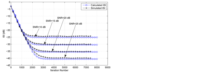
Figure 2. A comparison between the simulated and calculated ISI for the 16QAM source input going through channel1 for different SNR values. The averaged results were obtained in 100 Monte Carlo trials. The equalizer’s tap length and step-size parameter were set to 27 and 0.0002 respectively.

Figure 3. A comparison between the simulated and calculated ISI for the 16QAM source input going through channel1 for different step-size values. The averaged results were obtained in 100 Monte Carlo trials. The equalizer’s tap length was set to 27 and the .
.
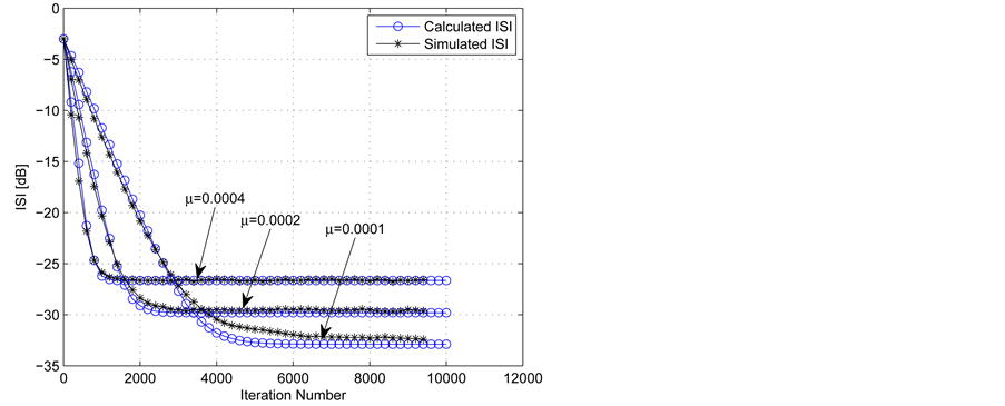
Figure 4. A comparison between the simulated and calculated ISI for the 16QAM source input going through channel1 for different step-size values. The averaged results were obtained in 100 Monte Carlo trials. The equalizer’s tap length was set to 31 and the .
.
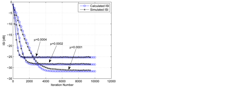
Figure 5. A comparison between the simulated and calculated ISI for the 16QAM source input going through channel2 for different step-size values. The averaged results were obtained in 100 Monte Carlo trials. The equalizer’s tap length was set to 41 and the .
.
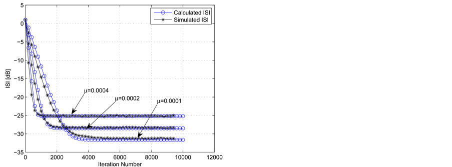
Figure 6. A comparison between the simulated and calculated ISI for the 16QAM source input going through channel3 for different step-size values. The averaged results were obtained in 100 Monte Carlo trials. The equalizer’s tap length was set to 41 and the .
.

Figure 7. A comparison between the simulated and calculated ISI for the 16QAM source input going through channel4 for different step-size values. The averaged results were obtained in 100 Monte Carlo trials. The equalizer’s tap length was set to 121 and the .
.
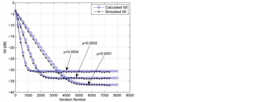
Figure 8. A comparison between the simulated and calculated ISI for the 16QAM source input going through channel5 for different step-size values. The averaged results were obtained in 100 Monte Carlo trials. The equalizer’s tap length was set to 13 and the .
.
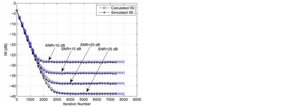
Figure 9. A comparison between the simulated and calculated ISI for the 16QAM source input going through channel5 for different SNR values. The averaged results were obtained in 100 Monte Carlo trials. The equalizer’s tap length and step-size parameter were set to 13 and 0.0002 respectively.
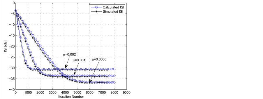
Figure 10. A comparison between the simulated and calculated ISI for the QPSK source input going through channel5 for different step-size values. The averaged results were obtained in 100 Monte Carlo trials. The equalizer’s tap length was set to 13 and the .
.

Figure 11. A comparison between the simulated and calculated ISI for the QPSK source input going through channel4 for different step-size values. The averaged results were obtained in 100 Monte Carlo trials. The equalizer’s tap length was set to 121 and the .
.
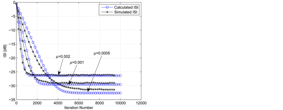
Figure 12. A comparison between the simulated and calculated ISI for the QPSK source input going through channel6 for different step-size values. The averaged results were obtained in 100 Monte Carlo trials. The equalizer’s tap length was set to 33 and the .
.
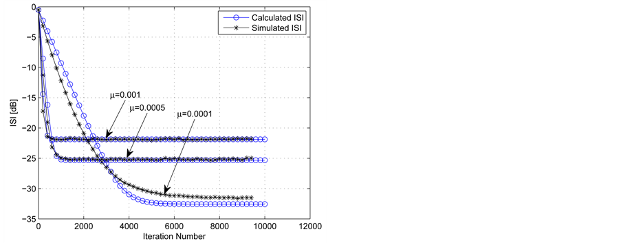
Figure 13. A comparison between the simulated and calculated ISI for the 16QAM source input going through channel6 for different step-size values. The averaged results were obtained in 100 Monte Carlo trials. The equalizer’s tap length was set to 33 and the .
.
enables the recovery of the transmitted sequence. A fast convergence time is obtained by choosing a higher value for the step-size parameter.
Next we turn to test the expression for the convergence time (13). For that purpose we use the following cases:
Case 1 (Figure 3 with ):
):
The simulated convergence time according to Figure 3 is approximately 1000 iterations. According to (13), the calculated convergence time is approximately 1059 iterations where the residual ISI was set to −27 dB.
Case 2 (Figure 3 with ):
):
The simulated convergence time according to Figure 3 is approximately 2000 iterations. According to (13), the calculated convergence time is approximately 2139 iterations where the residual ISI was set to −30 dB.
Case 3 (Figure 5 with ):
):
The simulated convergence time according to Figure 5 is approximately 1000 iterations. According to (13), the calculated convergence time is approximately 943 iterations where the residual ISI was set to −25 dB.
Case 4 (Figure 5 with ):
):
The simulated convergence time according to Figure 5 is approximately 1900 iterations. According to (13), the calculated convergence time is approximately 1814 iterations where the residual ISI was set to −28 dB.
Case 5 (Figure 8 with ):
):
The simulated convergence time according to Figure 8 is approximately 1000 iterations. According to (13), the calculated convergence time is approximately 1094 iterations where the residual ISI was set to −30 dB.
Case 6 (Figure 8 with ):
):
The simulated convergence time according to Figure 8 is approximately 4200 iterations. According to (13), the calculated convergence time is approximately 4414 iterations where the residual ISI was set to −35 dB.
Case 7 (Figure 12 with ):
):
The simulated convergence time according to Figure 12 is approximately 1000 iterations. According to (13), the calculated convergence time is approximately 903 iterations where the residual ISI was set to −25 dB.
Case 8 (Figure 12 with ):
):
The simulated convergence time according to Figure 12 is approximately 2000 iterations. According to (13), the calculated convergence time is approximately 1805 iterations where the residual ISI was set to −27.5 dB.
Based on the above mentioned cases (Case 1 - Case 8), there is a high correlation between the calculated (13) and simulated convergence time.
5. Conclusion
In this paper, we proposed for the real and two independent quadrature carrier input case, a closed-form approximated expression for the ISI as a function of time (or number of iteration number) valid during the entire stages of the iterative deconvolution process that depends on the SNR, on the step-size parameter used in the adaptation process, on the equalizer’s tap length, on the input signal statistics and on the channel’s power (which is measurable). The obtained expression is applicable for type of channels where the resulting ISI as a function of time can be described with an exponential model having a single time constant. Based on this new expression for the ISI as a function of time (or number of iteration number), the convergence time (or number of iteration number required for convergence) of the non-blind adaptive equalizer was obtained. Simulation results have shown a high correlation between the calculated (based on our new expression for the ISI as a function of time) and simulated ISI as a function of time. In addition, simulation results have shown that our new proposed expression for the convergence time produces approximately the same results as those obtained from the simu- lation.
Acknowledgements
We thank the Editor and the referee for their comments.
Cite this paper
MonikaPinchas, (2016) Convergence Curve for Non-Blind Adaptive Equalizers. Journal of Signal and Information Processing,07,7-17. doi: 10.4236/jsip.2016.71002
References
- 1. Pinchas, M. (2013) Residual ISI Obtained by Nonblind Adaptive Equalizers and Fractional Noise. Mathematical Problems in Engineering, 2013, Article ID: 830517, 7 p.
- 2. Pinchas, M. (2013) Two Blind Adaptive Equalizers Connected in Series for Equalization Performance Improvement. Journal of Signal and Information Processing, 4, 64-71.
http://dx.doi.org/10.4236/jsip.2013.41008 - 3. Godfrey, R. and Rocca, F. (1981) Zero Memory Non-Linear Deconvolution, Geophys. Prospect, 29, 189-228.
http://dx.doi.org/10.1111/j.1365-2478.1981.tb00401.x - 4. Shalvi, O. (1990) Weinstein E. New Criteria for Blind Deconvolution of Nonminimum Phase Systems (Channels). IEEE Transactions on Information Theory, 36, 312-321.
http://dx.doi.org/10.1109/18.52478 - 5. Pinchas, M. (2010) A Closed Approximated Formed Expression for the Achievable Residual Intersymbol Interference Obtained by Blind Equalizers. Signal Processing Journal (Eurasip), 90, 1940-1962.
http://dx.doi.org/10.1016/j.sigpro.2009.12.014 - 6. Pinchas, M. and Bobrovsky, B.Z. (2006) A Maximum Entropy Approach for Blind Deconvolution. Signal Processing (Eurasip), 86, 2913-2931.
http://dx.doi.org/10.1016/j.sigpro.2005.12.009 - 7. Haykin, S. (1991) Blind Deconvolution. In: Haykin, S., Ed., Adaptive Filter Theory, Prentice-Hall, Englewood Cliffs, Chapter 20.
- 8. Fiori, S. (2001) A Contribution to (Neuromorphic) Blind Deconvolution by Flexible Approximated Bayesian Estimation. Signal Processing, 81, 2131-2153.
http://dx.doi.org/10.1016/S0165-1684(01)00108-6 - 9. Bellini, S. (1986) Bussgang Techniques for Blind Equalization. IEEE Global Telecommunication Conference Records, 1634-1640.
- 10. Nikias, C.L. and Petropulu, A.P., Eds. (1993) Higher-Order Spectra Analysis A Nonlinear Signal Processing Framework. Prentice-Hall, Upper Saddle River, Chapter 9, 419-425.
- 11. Malik, G. and Sappal, A.S. (2011) Adaptive Equalization Algorithms: An Overview. International Journal of Advanced Computer Science and Applications (IJACSA), 2, 62-67.
- 12. http://www.academypublisher.com/proc/iscsct10/papers/iscsct10p256.pdf
- 13. Tucu, E., Akir, F. and Zen, A. (2013) A New Step Size Control Technique for Blind and Non-Blind Equalization Algorithms. Radioengineering, 22, 44.
- 14. Makki, A.H.I., Dey, A.K. and Khan, M.A. (2010) Comparative Study on LMS and CMA Channel Equalization. Information Society (i-Society), 2010 International Conference, 487-489.
- 15. Reuter, M. and Zeidler, J.R. (1999) Nonlinear Effects in LMS Adaptive Equalizers. IEEE Transactions on Signal Processing, 47, 1570-1579.
http://dx.doi.org/10.1109/78.765126 - 16. Pinchas, M. (2013) Residual ISI obtained by Blind Adaptive Equalizers and Fractional Noise. Mathematical Problems in Engineering, 2013, Research Article: 972174, 111.
Abbreviations
ISI: Intersymbol Interference
SNR: Signal to Noise Ratio
SISO: Single Input Single Output
FIR: Finite Impulse Response
QAM: Quadrature Amplitude Modulation
QPSK: Quadrature Phase Shift Keying