Journal of Signal and Information Processing
Vol. 3 No. 1 (2012) , Article ID: 17612 , 10 pages DOI:10.4236/jsip.2012.31002
Feature Extraction Techniques of Non-Stationary Signals for Fault Diagnosis in Machinery Systems
![]()
1Mechanical and Systems Research Laboratories, Industrial Technology Research Institute, Taiwan, China; 2Department of Mechanical Engineering, Chung Yuan Christian University, Taiwan, China.
Email: *jei0513@gmail.com
Received December 18th, 2011; revised January 20th, 2012; accepted February 5th, 2012
Keywords: Non-Stationary Signal; Short-Time Fourier Transform; Back Propagation Neural Network; Time Frequency Order Spectrum
ABSTRACT
Previously, fault diagnosis of fixed or steady state mechanical failures (e.g., pumps in nuclear power plant turbines, engines or other key equipment) applied spectrum analysis (e.g., fast Fourier transform, FFT) to extract the frequency features as the basis for identifying the causes of failure types. However, mechanical equipment for increasingly instant speed variations (e.g., wind turbine transmissions or the mechanical arms used in 3C assemblies, etc.) mostly generate non-stationary signals, and the signal features must be averaged with analysis time which makes it difficult to identify the causes of failures. This study proposes a time frequency order spectrum method combining the short-time Fourier transform (STFT) and speed frequency order method to capture the order features of non-stationary signals. Such signal features do not change with speed, and are thus effective in identifying faults in mechanical components under non-stationary conditions. In this study, back propagation neural networks (BPNN) and time frequency order spectrum methods were used to verify faults diagnosis and obtained superior diagnosis results in non-stationary signals of gearrotor systems.
1. Introduction
Fast Fourier transform can be used to analyze the frequency features of stationary signals, but it cannot clearly render signal characteristics of non-stationary signals with time variations. Time frequency analysis simultaneously considers time and frequency analysis methods, and can be used to analyze various frequencies at different times [1]. Dennis Gabor [2] proposed the short-time Fourier transform which can be seen as a fixed time frequency window transform with variable time frequenies, to show time and frequency variability in signals. Using the STFT to analyze non-stationary signals, Fadi et al. [3] obtained results superior to those obtained through FFT. Wang et al. [4] obtained feature extraction of time-frequency distribution images by using first-order time square and frequency square methods. Bie et al. [5] obtained the first-order grey square by thresholding in time-frequency gray-scale images. This method extracts time-frequency distribution image information, but easily captures excess noise and is thus unable to effectively obtain signal feature information.
Neural networks have superior learning and classification capabilities. In recent years, these methods have gradually replaced traditional diagnostic methods and obtained good diagnosis results. Rumelhart et al. [6] developed the learning ability of back-propagation neural networks to establish them as the most widely-used algorithm. For marine propulsion shaft systems, Kuo et al. [7] established a troubleshooting system taking fault types and spectral characteristics as the training samples for neural networks. The vibration acceleration spectrum is used as the neural network inputs and an increase in calculated output values for the trained neural network corresponds to a greater likelihood of failure. Wang et al. [8] used the different values of regression coefficients with neural networks to diagnose failures in rotating machinery.
This study proposes a method for mechanical fault diagnosis which combines the time-frequency order spectrum and back-propagation neural networks. A gear-rotor experimental platform was used to verify that this method could obtain superior diagnosis results for non-stationary signals.
2. Short-Time Fourier Transform
The short-time Fourier transform was used in this study for the feature extraction of non-stationary signals. The STFT provides a window function for movement along the time axis and obtains 2D function signals in the time and frequency domains. The partition FFTs were obtained at different times by fast Fourier transform of 2D function signals. The phase and energy of time-domain and frequency-domain were obtained by calculating the energy density spectrum of the partition FFTs.
To resolve the localization problem in the time domain, the time signal captured in the fast Fourier transform has a limited window function of time. When the signal is non-stationary, the analysis window is assumed to be stable over a short period of time, given the window function  for the sectional processing in signal function
 . Through the movement of the short-term window along the time axis, the local spectrum of the signal could be obtained. The signal is mapped into a two-dimensional function of time and frequency. In other words, at different times, the local spectrum can obtain time-varying characteristics in non-stationary signals. For signal
  in the period t, the STFT was defined as:
 (1)
(1)
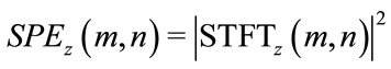
where  is a continuous function. Thus, the energy density of t can be defined as:
 (2)
(2)
In the calculation process, the above equation must be discrete. Assuming  is the k-th discrete signal, the discrete form of
  is:
is:
 (3)
(3)
where  and
and  respectively represent the indicators of time and frequency in the discrete samples. The signal
  is the length in the window function
 .
.
 (4)
(4)
3. Feature Extraction Method for Non-Stationary Signals
Although time-frequency analysis methods can be used to analyze non-stationary signals, the frequency features change with analysis time, making it difficult to meaningfully interpret frequency features. Therefore, this study proposes combining short-time Fourier transform with the speed frequency order method for feature extraction of non-stationary signals. Using the common vibration signals of rotating machinery as an example, the timefrequency spectrum of the vibration signal was obtained first by time-frequency analysis. The time-frequency order spectrum is obtained by dividing the instant timefrequency spectrum by the instant speed frequency. The magnitude variation of the time-frequency order spectrum could detect the failures. Figure 1 shows the following steps:
1) Acquire vibration signals of the rotating machinery.
2) Acquire the speed signal of the rotating machinery.
3) Obtain the time-frequency spectrum of the vibration signal by time-frequency analysis.
4) Calculate the instant time-frequency spectrum.
5) Calculate the instant speed frequency.
6) Divide the time-frequency spectrum by the instant time-frequency spectrum to obtain the time-frequency order spectrum, as shown in Figure 2.
Figure 3 shows the time-frequency analysis results; the simulated signal includes first and second order rotation frequencies. Although the figure shows the relationship between first and second order rotation frequencies as time changes, it cannot be qualitatively or quantitatively described. As shown in Figure 4, the proposed time-frequency order spectrum analysis can discern the first and second order rotation frequencies fixed on the time-frequency order spectrum, and also clearly show that the time-frequency characteristic frequencies do not change with time.
4. Back-Propagation Neural Network
Figure 5 shows a BPNN designed for fault diagnosis for non-stationary signals. It is composed of N nodes (S1 ~ SN) in the input layer, L nodes (H1 ~ HL) in the hidden layer and M nodes (O1 ~ OM) in the output layer. The input and output variables are arrayed into a vector as expressed by
(S1, S2, ~SN, O1, O1 ~ OM)(5)
where N input elements denote S1 ~ SN which represent the first time-frequency order spectrum to Nth time-frequency order spectrum, and M output elements denote O1 to OM which represent normal state, gear fault state, rotor fault state, etc.
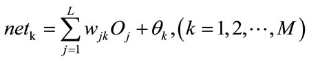
The connections between the input and hidden layers, and between the hidden and output layers are weighting coefficients wij and wjk, respectively. The input of the j-th neuron in the hidden layer can be expressed by
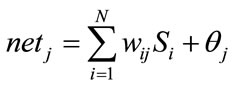 (6)
(6)
where si is the i-th input, wij is the weighting coefficient between the i-th neuron in the input layer and the j-th neuron in the hidden layer. Thus, the output of the j-th neuron in the hidden layer can be obtained by
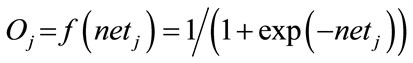 (7)
(7)
where  is the sigmoid function adopted as the activation function. The output of BPNN can be expressed
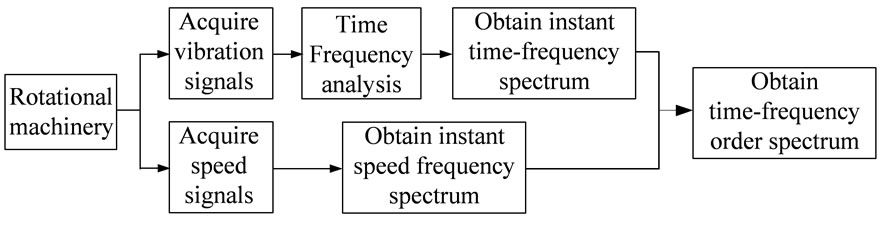
Figure 1. Time-frequency order spectrum method.
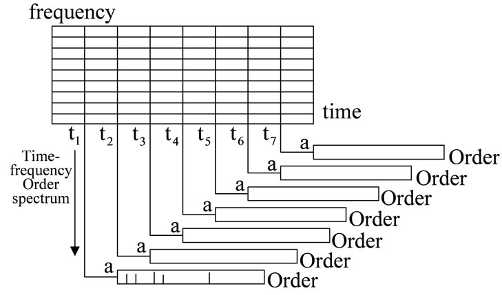
Figure 2. Time-frequency order spectrum.
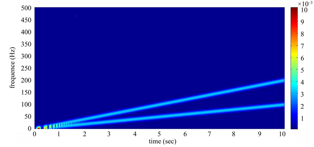
Figure 3. Short-time Fourier spectrum of the simulated signal.
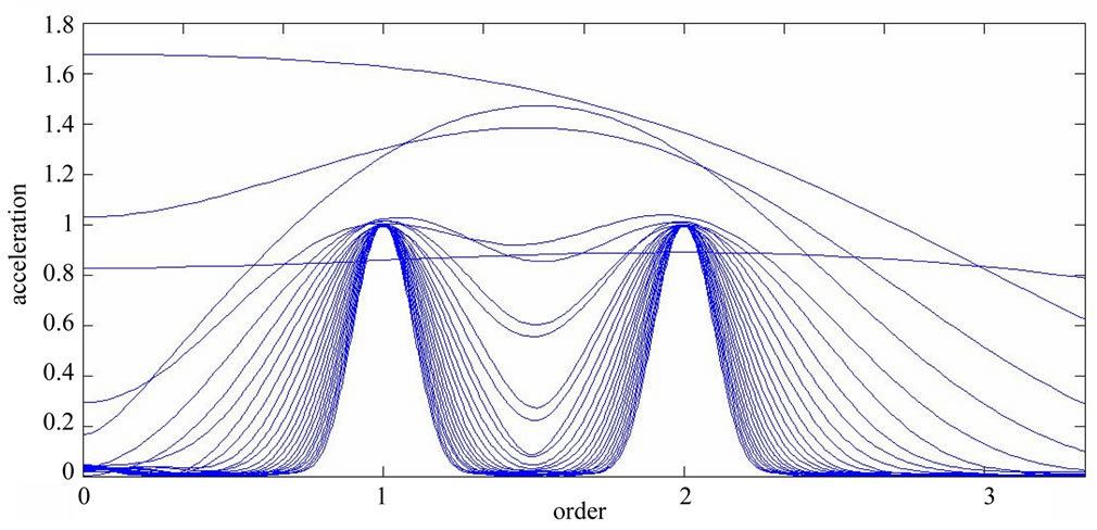
Figure 4. Time-frequency order spectrum of the simulated signal.
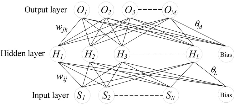
Figure 5. Structure of back-propagation neural network.
by
 (8)
(8)
where L is the neuron number in the hidden layer, wjk is the weighting coefficient between the j-th neuron in the hidden layer and the k-th neuron in the output layer. Then, the output Ok of the BPNN can be obtained by
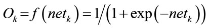 (9)
(9)
The BPNN is trained using the error between the actual output and the ideal output to modify wij and wjk until the output of BPNN is close to the ideal output with acceptable accuracy. Using the gradient descent method for error minimization, the correction increments of the weighting coefficients are defined as being proportional to the slope, related to the changes between the error estimator and the weighting coefficients as
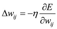 ,
,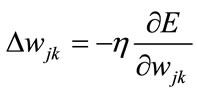 (10)
(10)
where  is the learning rate used for adjusting the increments of weighting coefficients and controls the convergent speed of the weighting coefficients.
  is the error estimator of the network and is defined by
 (11)
(11)
where Q is the total number of training samples.  is the ideal output of the p-th sample and
  is the actual output of the p-th sample. Substituting Equation (11) into Equation (10) and executing derivations gives the increments of weighting coefficients as
 (12)
(12)
for the output layer, and
 (13)
(13)
where  is the first derivation of
 . Therefore, in the training process, the weighting coefficients must be modified by
 (14)
(14)
until the error estimator E converges to an acceptable accuracy.
With network training complete, the values of timefrequency order spectrum are used to compute the trained weighting coefficients wij and wjk and obtain the network’s output values. Each output neuron represents a kind of state and the output value represents the degree of certainty for the corresponding state. A value is close to 1 indicates a higher probability for the given state.
5. Case Study
This study used a gear-rotor experimental platform with varying speeds to simulate different types of gear and rotor conditions including: gear normal, worn, broken teeth, gear unbalanced, normal state, misaligned, unbalanced and looseness (Table 1). The non-stationary signals were obtained from the experimental platform for use in failure diagnosis.
5.1. Varying Time Experiments on the Gear-Rotor Platform
As shown in Figure 6, the experiments simulate the vibration signal from a gear-rotor experimental platform (51 and 23 tooth gears) operating at different speeds. The LabView NI9401 DI/O was used as the interface for input signals to the circuit board, which dynamically controls the frequency to achieve the automation of speed variation. The operating process was as follows: The speed was dropped from 1600 rpm to 800 rpm within two seconds, and then increased to the final value of 1500 rpm. The non-stationary speed curve is shown in Figure 7. The NI9234 DAQ simultaneously acquired the vibration signals and speed signals at a sampling frequency of 6400 Hz.
In this experiment, non-stationary signals are measured under 8 different kinds of conditions, with 20 samples taken for each condition for a total of 160 samples. In the time-domain, the signals of all samples were subjected to STFT. Thus, the first 200 orders of the total signal characteristics in the time-frequency order spectrum are obtained through the non-stationary time-frequency extrac-
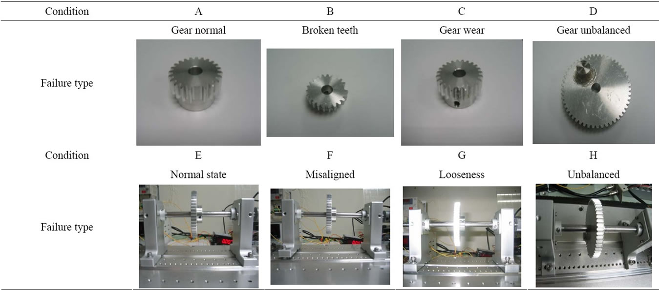
Table 1. Gear-rotor experimental platform failure conditions.

Figure 6. Gear speed change simulation platform.
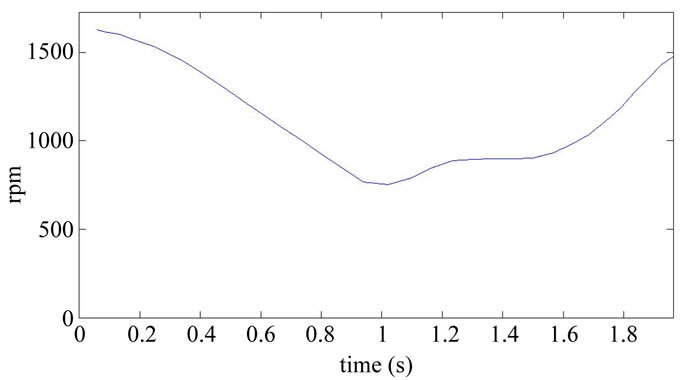
Figure 7. Non-stationary speed curve.
tion technique.
5.2. Non-Stationary Signal Feature Extraction
Table 1 shows the conditions of eight different vibration signals used in the experiment. Figures 8(a) and (e) respectively show conditions A and B of the platform of the gear-rotor signal in the time domain for all conditions. Figures 8(b) and (f) respectively show the spectra of the fast Fourier transform frequency, and Figures 8(c) and (g) respectively show the frequency of spectrum images obtained from STFT. The spectrum images were taken every 0.1 second so that the time-frequency order spectrum is obtained by dividing the instant time-frequency spectrum by the instant speed frequency. All instant time-frequency order spectra were superimposed and then averaged to obtain the time-frequency order spectrum, represented respectively in Figures 8(d) and (h). The operational statuses for signals C ~ H were similarly measured and analyzed, and are respectively depicted in Figures 9-11. For the eight calculated time-frequency order spectra, the conditions of B and C at the 23th order display significant amplitude, respectively indicating broken teeth and wear on the gear. Condition D at the 51th order shows significant amplitude, indicating significant gear imbalance. Lastly, the rotor conditions E to H generate varying amplitudes in order 1st ~ 3rd.
5.3. Back-Propagation Neural Network Diagnosis Results
This study used STFT with non-stationary signal extraction techniques to obtain the time-frequency order spectrum. Next, the value of the extracted features was inputted to the back-propagating neural networks to obtain the failure diagnosis as follows:
1) Figure 12 illustrates the structure of back-propagating neural networks used in this study. The time-frequency order spectrum is used as input, and the input neuron count a is defined as 200 while the hidden level neuron count is 250.
2) In the experiment, conditions A ~ H (Table 1) can be used in the neural network, with different respective assembled outputs as follows: [1 0 0 0 0 0 0 0], [0 1 0 0 0
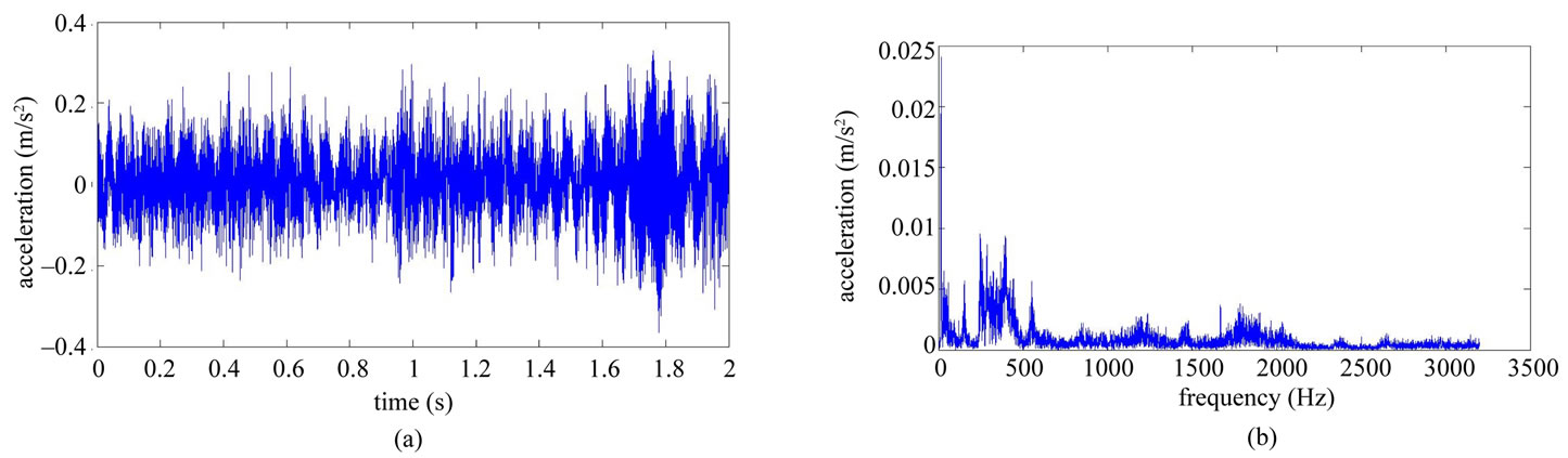
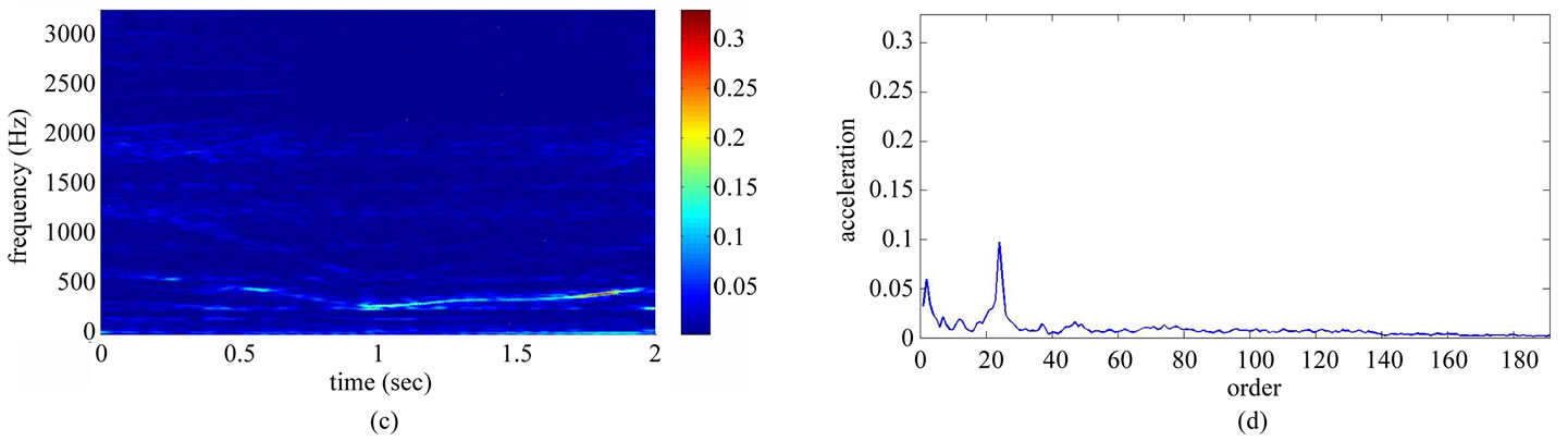
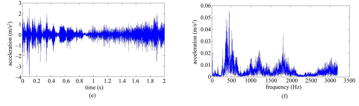
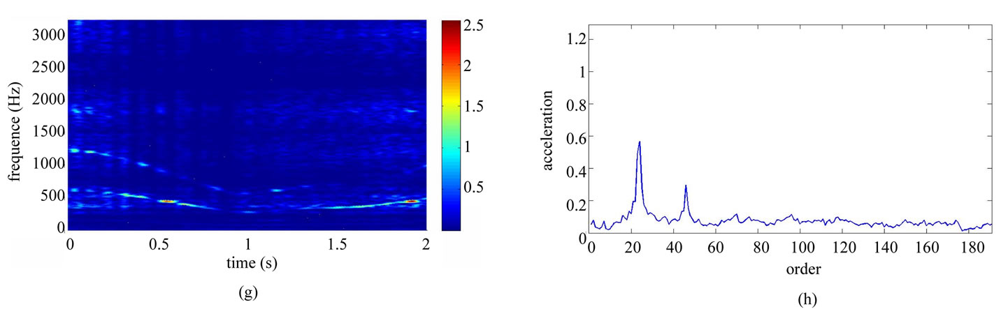
Figure 8. Non-stationary signal feature extraction for conditions A and B. (a) Time-domain signal (condition A); (b) Frequency spectrum (condition A); (c) STFT time-frequency spectrum (condition A); (d) STFT time-frequency order spectrum (condition A); (e) Time-domain signal (condition B); (f) Frequency spectrum (condition B); (g) STFT time-frequency spectrum (condition B); (h) STFT time-frequency order spectrum (condition B).
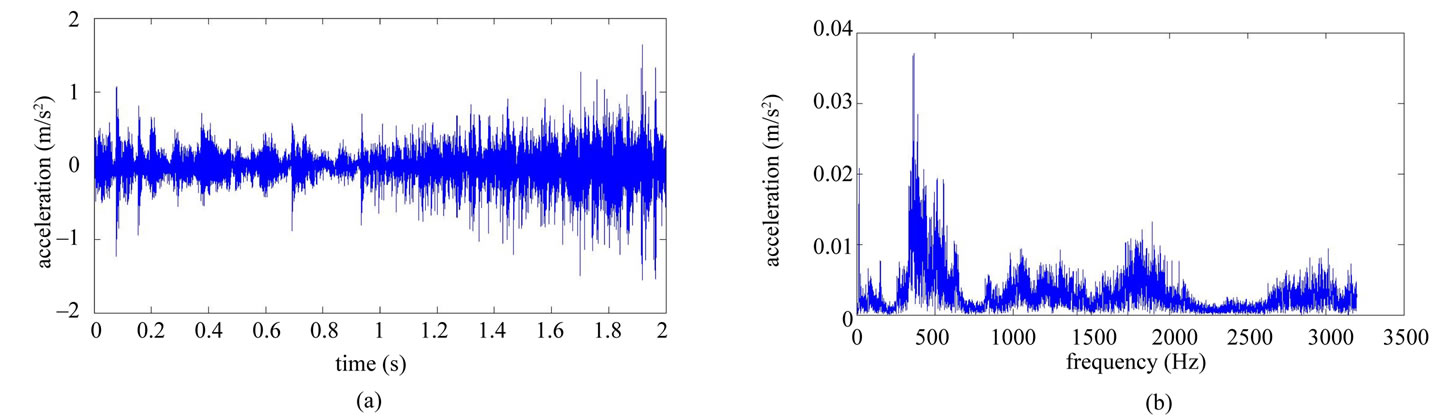
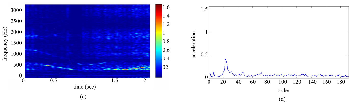
Figure 9. Non-stationary signal feature extraction for conditions C and D. (a) Time-domain signal (condition C); (b) Frequency spectrum (condition C); (c) STFT time-frequency spectrum (condition C); (d) STFT time-frequency order spectrum (condition C); (e) Time-domain signal (condition D); (f) Frequency spectrum (condition D); (g) STFT time-frequency spectrum (condition D); (h) STFT time-frequency order spectrum (condition D).
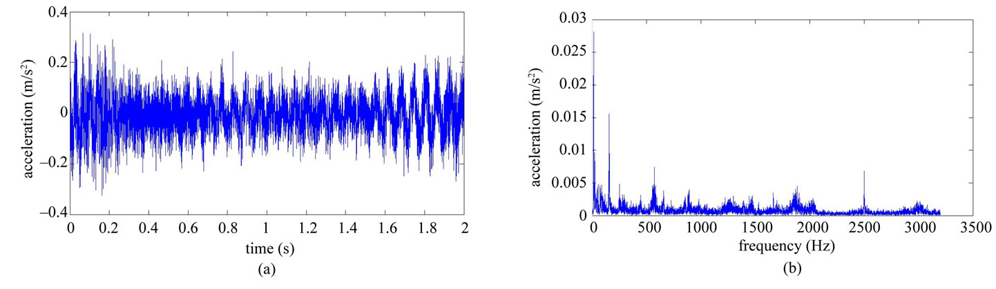
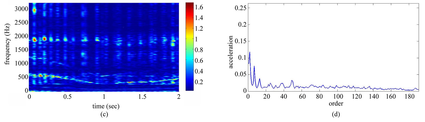
Figure 10. Non-stationary signal feature extraction for conditions E and F. (a) Time-domain signal (condition E); (b) Frequency spectrum (condition E); (c) STFT time-frequency spectrum (condition E); (d) STFT time-frequency order spectrum (condition E); (e) Time-domain signal (condition F); (f) Frequency spectrum (condition F); (g) STFT time-frequency spectrum (condition F); (h) STFT time-frequency order spectrum (condition F).
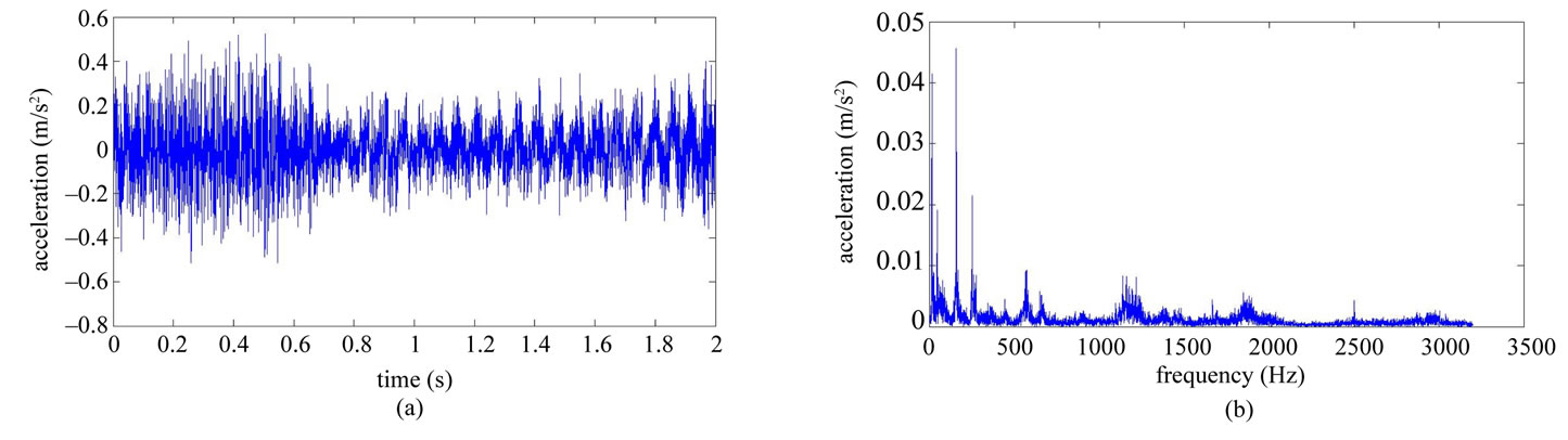
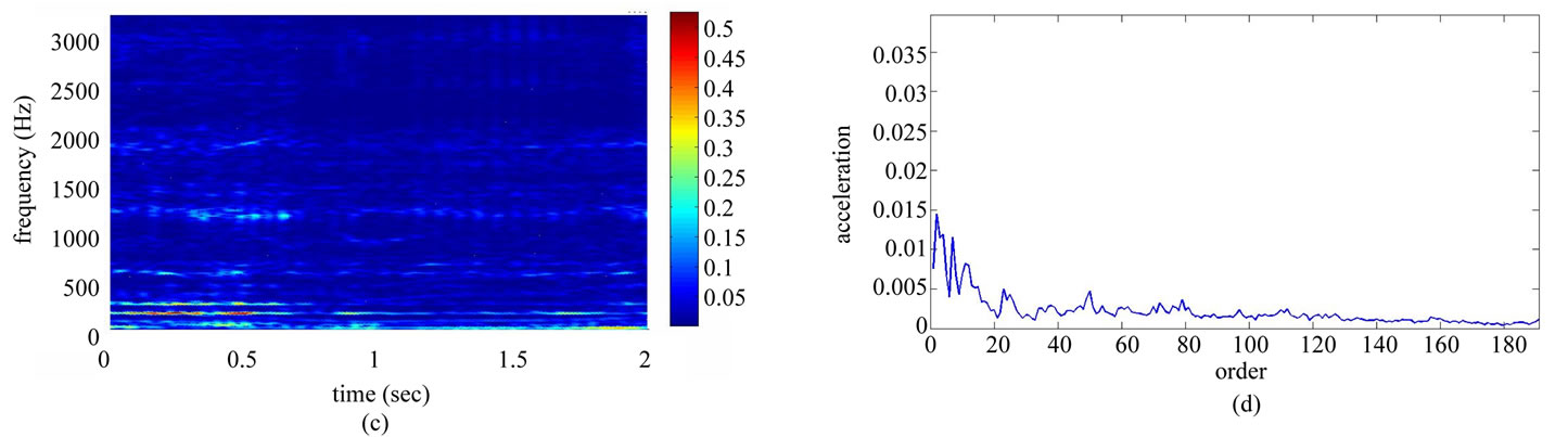
Figure 11. Non-stationary signal feature extraction for conditions G and H. (a) Time-domain signal (condition G); (b) Frequency spectrum (condition G); (c) STFT time-frequency spectrum (condition G); (d) STFT time-frequency order spectrum (condition G); (e) Time-domain signal (condition H); (f) Frequency spectrum (condition H); (g) STFT time-frequency spectrum (condition H); (h) STFT time-frequency order spectrum (condition H).
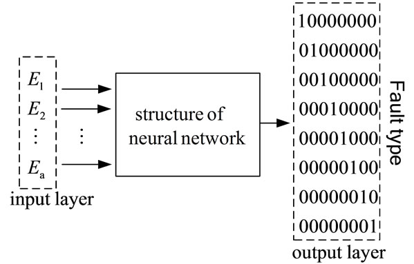
Figure 12. Time-frequency order spectrum neural network training.
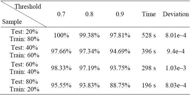
Table 2. STFT time-frequency order spectrum + BPNN recognition accuracy.
0 0 0], [0 0 1 0 0 0 0 0], [0 0 0 1 0 0 0 0], [0 0 0 0 1 0 00], [0 0 0 0 0 1 0 0], [0 0 0 0 0 0 0 0 1 0] and [0 0 0 0 0 0 0 0 0 1].
3) Of the 20 samples each for A ~ H (160 samples total), sample assemblies were randomly chosen for training and testing, with the four assemblies as follows: First, 20% training and 80% testing (32 training samples, 128 test samples); second, 40% training and 60% testing (64 training samples, 96 test samples); third, 60% training and 40% testing (96 training samples, 65 test samples) and finally, 80% training samples and 20% testing samples (128 training samples, 32 test samples).
4) Diagnosis results: To verify the STFT time-frequency order spectrum network output values, this study took the values of 0.7, 0.8 and 0.9 as the criteria for the determination value, as shown in Table 2. Among all these numbers, if the threshold value of 0.7 is correct, the accuracy is high but the low threshold would make it prone to error. The threshold of 0.9 is too high, resulting in low accuracy. Therefore, this study recommends the setting threshold value as 0.8.
6. Conclusions
Combining the time-frequency order spectrum with neural networks obtains good recognition results for all types of non-stationary signals. The conclusions as follows:
1) In the proposed method, the time-frequency order 2) Under different conditions, the proposed time-frequency order spectrum can fix features such that speed will not change during the time period. Thus, the magnitude of changes in feature order can be observed in nonstationary signals, allowing for the recognition of anomalies.
3) The proposed combination of the time-frequency order spectrum and back-propagation neural networks diagnoses failures with an accuracy rate of 93% or higher using a ratio of 20:80 for training to test samples. All the testing samples reduce the required training time to 196 seconds.
REFERENCES
- C. F. Xu and G. K. Li, “Practical Wavelet Method,” Huazhong University of Science & Technology Press Co., Taichung, 2004, pp. 46-48.
- G. Dennis, “Theory of Communications,” Journal of the Institution of Electrical Engineers, Vol. 93, No. 4, 1946, pp. 429-457.
- F. Al-Badourl, L. Chedect and M. Suna, “Non-Stationary Vibration Signal Analysis of Rotating Machinery via Time-Frequency and Wavelet Techniques,” Information Sciences Signal Processing and Their Applications, Kuala Lumpur, 10-13 May 2010, pp. 21-24.
- Z. H. Wang and Y. H. Yu, “Fault Diagnosis of Diesel Engine Exhaust Valve Leakage Using Time Frequency Analysis Method,” Journal of Wuhan University of Technology, Vol. 32, No. 4, 2008, pp. 645-648.
- F. F. Bie, F. T. Wang and F. X. Lu, “Intelligent Diagnosis of Reciprocating Compressor Based on Local Wave Time-Frequency Spectra Processing,” Transactions of the Chinese Society for Agricultural Machinery, Vol. 38, No. 9, 2007, pp. 159-162.
- D. E. Rumelhart, G. E. Hinton and R. J. Williams, “Learning Representations by Back-Propagating Errors,” Nature, Vol. 323, No. 6088, 1986, pp. 533-536. doi:10.1038/323533a0
- H. C. Kuo, L. J. Wu and J. H. Chen, “Neural-Fuzzy Fault Diagnosis in a Marine Propulsion Shaft System,” Journal of Materials Processing Technology, Vol. 122, No. 1, 2000, pp. 12-22. doi:10.1016/S0924-0136(01)01157-8
- C. C. Wang, Y. Kang, P. C. Shen, Y. P. Chang and Y. L. Chung, “Applications of Fault Diagnosis in Rotary Machinery by Using Time Series Analysis with Neural Network,” Expert System With Application, Vol. 37, No. 2, 2010, pp. 1696-1702. doi:10.1016/j.eswa.2009.06.089
NOTES
*Corresponding author.