ABSTRACT

This paper presents and compares four mathematical models with unique spatial effects for a prey-predator system, with Tetranychus urticae as prey and Phytoseiulus persimilis as predator. Tetranychus urticae, also known as two-spotted spider mite, is a harmful plant-feeding pest that causes damage to over 300 species of plants. Its predator, Phytoseiulus persimilis, a mite in the Family Phytoseiidae, effectively controls spider mite populations. In this study, we compared four mathematical models using a numerical simulation. These models include two known models: self-diffusion, and cross-diffusion, and two new models: chemotaxis effect model, and integro diffusion model, all with a Beddington-De Angelis functional response. The modeling results were validated by fitting experimental data. Results demonstrate that interaction scheme plays an important role in the prey-predator system and that the cross- diffusion model fits the real system best. The main contribution of this paper is in the two new models developed, as well as the validation of all the models using experimental data.

Keywords:

Two-Spotted Spider Mite, Phytoseiulus persimilis, Mathematical Model, Prey-Predator System

1. Introduction

The two-spotted spider mite, Tetranychus urticae, is a species of plant-feeding mites generally considered to be a pest. It is the most widely known member of the Family Tetranychidae and is a harmful pest in greenhouses and on field-grown crops. Previous reports have stated that Tetranychus urticae infests over 300 species of plants, including ornamental plants such as arborvitae, azalea, camellia, citrus, evergreens, hollies, ligustrum, pittosporum, pyracantha, rose, and viburnum; fruit crops such as blackberries, blueberries, and strawberries; and vegetable crops such as tomatoes, squash, eggplant, and cucumber [1] .

Insects have three pairs of legs and three body regions (head, thorax, abdomen), but throughout most life stages, spider mites have four pairs of legs and one body region. Tetranychus urticae is distinguishable by two large dark green spots on the dorsal area of the abdomen. Depending on the host plant and other environmental factors, such as temperature and light, the color of Tetranychus urticae varies from light green, dark green, brown, black, and orange [2] . The population of Tetranychus urticae completes a generation every 7 - 10 days, depending on the temperature. They have five stages of development: egg, larva, protonymph, deutonymph, and adult [3] .

Predators beneficially regulate spider mite populations. Five species of spider mite predators are commercially available in the United States for crop protection: Phytoseiulus persimilis, Mesoseiulus longipes, Neoseiulus californicus, Galendromus occidentalis, and Amblyseius fallicus. Predatory mites are distinguishable from spider mites due to longer legs, a more active life, and a faster pace of movement. Predators are often red or orange in color [1] . Phytoseiulus persimilis, the most common predator of all stages of mites, is thought to originate from the Mediterranean or South America, but, since the 1960s, it has been established worldwide as a biological control agent, primarily for two-spotted spider mites. Phytoseiulus persimilis tolerates hot climates if relative humidity remains between 60 and 90 percent. This predator can consume 20 eggs or five adults daily; females consume much more than immature and adult males. Each female can produce 60 eggs in her lifetime. Phytoseiulus persimilis has five developmental stages: egg, nonfeeding larva, protonymph, deutonymph, and adult [3] . However, it often needs to be reintroduced because it relies exclusively on mites for food, eventually consuming all available prey. This beneficial mite is commercially available and commonly released against Tetranychus urticae [1] .

Previous work has attempted to determine biological mechanisms, including dispersal, underlying mechanism of the spider mite-Phytoseiulus persimilis interaction. When diffusion is introduced into a prey-predator system, both species attain uniform distributions in the domain after certain time. Diffusion acts as a stabilizer in a reaction-diffusion system [4] . Under certain conditions, however, diffusion can destabilize the process, leading to non-uniform distribution in a prey-predator system. This destabilization is known as diffusion-driven instability [5] .

Similar to predator interference and relative diffusion, another factor, called prey- taxis, introduce instability into this domain, and leading to the formation of spatial patterns. In the Lotka-Volterra logistic prey-predator model with prey-taxis, Sapoukhina et al. [6] demonstrated that “predators respond to the heterogeneity of the prey density by accelerating toward the localities where the prey is abundant, resulting in predator aggregation.”

Phytoseiulus persimilis responds to odors released from leaves infested by Tetranychus urticae. Sabelis and Weel [7] discussed behavioral mechanisms of this predator by odor perception and how it contributes to prey identification. They observed the predators’ walking paths in still air and in an air stream uniformly permeated with or without prey-related odor stimuli. According to Sabelis and Weel, “the anemotactic responses observed are therefore both odour-conditioned and (feeding) state-dependent.” An anemotactic response of starved predators may help them find clusters of spider mite colonies [8] .

This paper presents and compares four prey-predator models with distinctive spatial effects as they apply to a two-spotted spider mite and Phytoseiulus persimilis system. The paper is organized as follows. Section 2 presents the four models, i.e. self-diffusion model, cross-diffusion model, chemotaxis effect model, and integro-diffusion model for a Tetranychus urticae and Phytoseiulus persimilis prey-predator dynamic system. Section 3 presents simulation results, and Section 4 compares experimental data with simulated data from various models. Section 5 discusses numerical simulation and model validation.

2. Mathematical Models

The dynamic relationship between predator and prey is a central ecological matter and a primary concern when modeling prey-predator interactions. A significant component of the prey-predator relationship is the functional response, which indicates the average number of prey killed per predator per unit of time. Two types of functional response are common: prey-dependent and predator-dependent. Prey-dependent implies that the functional response depends only on prey density; in a predator-dependent response, the function of response depends on both prey and predator densities. In the literature, the prey-dependent function has served as the basis for predator-prey theory, such as Holling’s Type II functional response [9] . However, researchers have argued that when predators must search for food and then share or compete for food, the functional response should depend on both prey and predator densities. Considerable evidence suggests that predator-dependent functional responses occur quite frequently in laboratory as well as in natural systems [10] . One of the most popular functional responses is the Beddington-DeAngelis functional response [11] [12] , originally proposed

by Beddington [13] and DeAngelis et al. [14] . The function is noted as.

This paper employs the Beddington-DeAngelis response function [11] [12] [13] [14] under an assumption that the predator Phytoseiulus persimilis must search for food. The logistic growth function is also employed for a prey system. The basic model is presented in Equation (1):

(1)

where

: spider mite and Phytoseiulus persimilis densities at time t, respectively

r: intrinsic growth of spider mites

K: carrying capacity of spider mites

e: conversion rate of prey to predator

d: death rate of Phytoseiulus persimilis

a: maximum consumption rate

b: saturation constant

c: factor to scale the impact of predator interference.

Let.

After manipulation, the following polynomial form is obtained:

(2)

This dynamic relationship is demonstrated in Figure 1 and Figure 2 which present two snapshots of dynamic simulation with the parameter α = 0.5, δ = 0.3, γ = 0.8 and an initial density for prey of 0.209 while the initial density for predator is 0.2203; maximum simulation time is 2000. Figure 1(a) and Figure 2(a) demonstrate the density of prey and predator changes through time, while the red line represents of density of prey, and the blue line represents the density of predator. Figure 1(b) and Figure 2(b) demonstrate the trajectory of the dynamical system.

According to Figure 1 and Figure 2, beta is correlated to the system stability. The system is unstable as shown in Figure 1 when β = 0.038 and the system is stable when β = 0.066.

This paper fits the dynamic system (2) into four models: self-diffusion model and cross-diffusion model which are based on existing formulations, and chemotaxis effect model and integro diffusion model which are part of the contribution of this paper. These models are presented in the following sections.

2.1. Self-Diffusion Model

The tendency for a species to move in the direction of lower species density is called

self-diffusion [15] . A general form of a self-diffusion model for a prey and predator system is presented as follows:

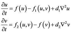(3)

where:

: birth rate function of prey

: death rate function of predator

: interaction function effect on the decrease of prey

: interaction function effect on the increase of predator

d₁: self-diffusion coefficient for prey

d₂: self-diffusion coefficient for predator

: usual Laplacian operator in two dimensions.

For the Beddington-DeAngelis response function and logistic growth function, the corresponding polynomial form becomes:

(4)

2.2. Cross-Diffusion Model

Although the self-diffusion model demonstrates that the movement within a given species is independent of other species, prey may recognize predators and respond by moving away to avoid capture by predators in predator-prey systems. However, if predators recognize prey, this recognition may affect the rate or direction of their movement, thereby helping the predators find prey. This phenomenon, known as cross-diffusion, has recently received significant attention, as described in [16] [17] [18] [19] . Value of the cross-diffusion coefficient may be positive, negative, or zero. A positive cross-diffusion coefficient denotes species movement in the direction of lower concentration of another species. A negative cross-diffusion coefficient indicates that one species tends to diffuse in the direction of higher concentration of another species.

The general form of a cross-diffusion model for prey-predator interactions is presented as follows:

(5)

where:

: birth rate function of prey

: death rate function of predator

: interaction function effect on the decrease of prey

: interaction function effect on the increase of predator

d₁₁ and d₂₂: self-diffusion coefficients of prey and predator, respectively

d₁₂and d₂₁: cross diffusion coefficients of predator and prey, respectively.

If d₁₂ > 0 and d₂₁ < 0, then the prey species tends to diffuse in the direction of lower concentration of the predator species and the predator species tends to diffuse in the direction of higher concentration of the prey species. Using the Beddington-DeAngelis response function and logistic growth function, the corresponding polynomial form becomes:

(6)

2.3. Chemotaxis Effect Model

A large number of insects, animals, and humans rely on smell to convey information between species members. Predatory mites respond to volatile chemicals released by plants infested with spider mites, as shown in experiments using Y-tube olfactometers and chemical analyses [5] . Previous research work has investigated the attraction mechanism between Phytoseiulus persimilis and herbivore-induced plant volatiles [20] [21] [22] [23] . For example, Michiel van Wijk confirmed that P. persimilis identifies chemical compounds in odor mixtures but the predators possess a limited ability to identify individual spider mite-induced plant volatiles in odor mixtures. Therefore, predatory mites have to learn to respond to prey-associated odor mixtures [23] . This section models this chemically-directed movement, or chemotaxis effect.

The predator-prey model with chemotaxis effect can be written as:

(7)

where:

: population density of prey

: population density of predator

: velocity of predators

: presence of a gradient in an attractant

: function of the attractant concentration

d₃: effect of social behavior

T: sensitivity coefficient of predators to heterogeneous density distribution of prey

2.4. Integro Diffusion Model

Integro-differential equations (IDEs) share continuous-space and continuous population assumptions of partial-differential equation (PDE) models. The PDE model focuses on localized movement (diffusion) of individuals, while IDE models focus on long- range movement. In this case, both prey and predator can move a long distance.

The predator-prey model with IDE can be written as:

(8)

Equation (8) considers movement from all points in space D (labeled y in the integral) to point x. T is the dispersal time of each species, and μ is a species parameter describing the diffusivity, or rate of dispersal, of each population. Movement rate, assumed to vary with distance, is described by kernel function K₁ and K₂. Kernel function defines how movement rate decreases with distance, thus offering greater flexibility than the PDE model. Therefore, predation can occur over a variety of scales instead of being a local event.

3. Numerical Simulation

In this section, dynamic simulations are performed with the four discussed models. The simulation is performed on a two-dimensional lattice with 100 × 100 cells. Spacing between each lattice cell was 1.25 unit distance, and the timing step was 0.05. Laplacian diffusion was calculated using finite difference, and Neumann boundary conditions were employed. The parameter used [15] was α = 0.5, β = 0.128, γ = 0.8, δ = 0.3, d₁₁ (d₁) = 0.01, d₂₂ (d₂) = 1, d₁₂ = 0.005, and d₂₁ = −0.001. Additional parameters for the chemotaxis effect model were d₃ = 0.005, T = 0.01, for integro diffusion model were μ = 0.051, T = 2.5.

3.1. Prey and Predator Density Simulation

Prey and predator densities were compared at fixed locations of (50, 50) and (90, 90) within a 100 × 100 grid. The simulation ran 10,000 iterations with initial prey density 0.5 and predator density 0.2. Results of the self-diffusion model, cross-diffusion model, chemotaxis effect model, and integro diffusion model are shown in Figures 3-6, respectively. In all four figures, the left subfigure (a) represents prey and predator densities at the location (50, 50) and the right subfigure (b) represents these densities at the location (90, 90).

Simulation results in Figures 3-6 show that the chemotaxis effect model differs significantly from the other three models. The chemotaxis effect system did not achieve steady state by 10,000 iterations, while the other three dynamic systems achieved steady state at approximately 4000 - 6000 iterations. The reason for this could be predatory

mites move faster toward the higher density of prey area when attraction odors are present for predatory mites, thereby weakening system stability.

3.2. Pattern Simulation

This section presents simulated patterns of formation among models. Using stable state as the initial condition, simulations were run with 0, 100,000, and 20,000 iterations. Corresponding results are shown in subfigure (a), subfigure (b), and subfigure (c) of Figures 7-10, respectively. Simulated results for self-diffusion, cross-diffusion, chemotaxis effect, and integro diffusion models are shown in Figures 7-10, respectively.

From Figures 7-10, it could be concluded that different spatial effect played important role towards the dynamic system. Using the chemotaxis effect model shows a larger range of density distributions of prey and predator than that of the other three models when they all began from the same steady state. For instance, after 20,000 iterations, the difference of density distribution of prey is around 0.45 for chemotaxis effect model while that for other models is around 0.0045, and the density distribution difference of

predator is about 0.05 for chemotaxis effect model while that of predator for other models is about 0.0005. This indicates that chemotaxis introduces more instability into the model. On the other side, the pattern for the integro diffusion model differed significantly from the other models, which is consistent with the model assumption that prey and predator system has long-range interaction during their movement. The simulation results verified the assumption of different spatial effect models and confirmed that different interaction scheme plays an important role in this prey-predator system.

4. Validation

4.1. Introduction of the Experiment

This experiment, conducted by the entomology department at Kansas State University, was carried out on 24 individually-potted lima beans plants set in 8 × 3 arrays, with Phytoseiulus persimilis as predator and Tetranychus urticae as prey. The experiment lasted four weeks, and the total number of two-spotted spider mites and predator were counted every six days. Table 1 lists the total number of observed prey (Tetranychus urticae) and predator numbers in 24 days.

4.2. Comparison of Total Number of Prey and Predator

This section compares the number of two-spotted spider mites and its predator using a simulated model with the experimental (actual) observations. Parameters in Equation (1) for simulation were α = 20, b = 105, c = 45, d = 0.3, e = 0.25, r = 0.38, K = 800.

Simulation results are shown in Figures 11-14, where the dotted curve represents actual data from the experiment and the solid curve represents the number of prey and predator calculated from the simulated models. The number of prey comparison is presented on the subfigure (a) while the number of predator comparison is presented in the subfigure (b) of each figure.

From Figure 11 to Figure 14, we can see that the total number of prey has good fit while the total number of predator does not have the same good fit. In order to compare the results numerically, we performed statistical analysis comparing the simulation results with observations. This analysis employs Root Mean Squared Error (RMSE). RMSE is a measure of how close a fitted line is to data points. The use of RMSE is very common and makes an excellent general purpose error metric for numerical predictions. The statistical analysis is presented in Table 2 and Table 3.

Results show that the cross-diffusion model fits the two-spotted spider mite system best, with the smallest RMSE compared to the other three models for prey and predator number prediction. The integro diffusion model had the largest RMSE for prey number prediction while the chemotaxis effect model had the largest RMSE for predator number prediction.

5. Conclusions

This paper presented and analyzed four mathematical models with the Beddington- DeAngelis functional response [11] [12] [13] [14] for Tetranychus urticae and Phytoseiulus persimilis prey-predator system. The four models were the self-diffusion model, the cross-diffusion model, the chemotaxis effect model, and the integro diffusion model. Simulation results were shown using a numerical example. One conclusion obtained from the results is that different spatial effects impact the prey-predator distribution, since the integro-diffusion model exhibit a significantly differently pattern than the other three models.

Another conclusion that could be made is that, the two proposed models were theoretically reasonable. According to the simulation, the chemotaxis effect model was not as stable as the other three models, affirming that predator mites move faster and further when presented with attracting odors, thereby reducing system stability. The chemotaxis effect model lack of stability was also derived from the pattern formation simulation result. The result shows the range of density distribution of the chemotaxis effect model was much larger than that of the other three models when all models began from an identical steady state. On the other hand, the pattern for the integro diffusion model differed from the other models, which is consistent with the model assumption that prey and predator has long-range interaction during their movement.

In the validation process, results showed that all four models have good fit with the real system, with the cross-diffusion model having the best fit. For a future research, we plan to develop an agent-based model [24] [25] [26] to simulate interactions and predict the key parameters in order to offer suggestions on controlling the number of predators. Also, future expansion of this research can consider applying optimal control theory [27] [28] to provide decision makers with better policies of controlling the population of the two-spotted spider mites. Spatial games which have been adopted to analyze various structure of populations [29] [30] , also present a future expansion of our research.

Cite this paper

Kuang, Y., Ben- Arieh, D., Zhao, S.N., Wu, C.-H., Margolies, D. and Nechols, J. (2017) Mathematical Model for Two-Spotted Spider Mites System: Verification and Validation. Open Jour- nal of Modelling and Simulation, 5, 13-31. http://dx.doi.org/10.4236/ojmsi.2017.51002

References

- 1. Fasulo, T.R. and Denmark, H.A. (2009) Two-Spotted Spider Mite, Featured Creatures. University of Florida Institute of Food and Agricultural Sciences, Gainesville.
- 2. Chakraborty, A., Singh, M. and Ridland, P. (2009) Effect of Prey-Taxis on Biological Control of the Two-Spotted Spider Mite—A Numerical Approach. Mathematical and Computer Modelling, 50, 598-610.
https://doi.org/10.1016/j.mcm.2009.01.005 - 3. Nachappa, P., Margolies, D., Nechols, J. and Campbell, J. (2011) Variation in Predator Foraging Behaviour Changes Predator—Prey Spatio-Temporal Dynamics. Functional Ecology, 25, 1309-1317.
https://doi.org/10.1111/j.1365-2435.2011.01892.x - 4. Chakraborty, A., Singh, M., Lucy, D. and Ridland, P. (2009) A Numerical Study of the Formation of Spatial Patterns in Two-Spotted Spider Mites. Mathematical and Computer Modelling, 49, 1905-1919.
https://doi.org/10.1016/j.mcm.2008.08.013 - 5. Murray, J.D. (2002) Mathematical Biology. 3rd Edition, Springer-Verlag, Berlin.
- 6. Sapoukhina, N., Tyutyunov, Y. and Arditi, R. (2003) The Role of Prey-Taxis in Biological Control: A Spatial Theoretical Model. The American Naturalist, 162, 59-76.
https://doi.org/10.1086/375297 - 7. Sabelis, M.W. and Van der Weel, J.J. (1993) Anemotactic Responses of the Predatory Mite, Phytoseiulus persimilis Athias-Henriot, and Their Role in Prey Finding. Experimental & Applied Acarology, 17, 521-529.
https://doi.org/10.1007/BF00058895 - 8. Osborne, L.S., Ehler, L.E. and Nechols, J.R. (1985) Biological Control of the Two-Spotted Spider Mite in Greenhouses. Bulletin (Technical), University of Florida, Central Florida Research Center, Vol. 85, 1-8.
- 9. Holling, C.S. (1965) The Functional Response of Predator to Prey Density and Its Role in Mimicry and Population Regulation. The Memoirs of the Entomological Society of Canada, 97, 5-60.
- 10. Fan, M. and Kuang, Y. (2004) Dynamics of a Non-Autonomous Predator-Prey System with the Beddington-DeAngelis Functional Response. Journal of Mathematical Analysis and Applications, 295, 15-39.
https://doi.org/10.1016/j.jmaa.2004.02.038 - 11. Haque, M. (2011) A Detailed Study of the Beddington-DeAngelis Predator-Prey Model. Mathematical Biosciences, 234, 1-16.
https://doi.org/10.1016/j.mbs.2011.07.003 - 12. Li, H.Y. and Takeuchi, Y. (2011) Dynamics of the Density Dependent Predator-Prey System with Beddington-DeAngelis Functional Response. Journal of Mathematical Analysis and Applications, 374, 644-654.
https://doi.org/10.1016/j.jmaa.2010.08.029 - 13. Beddington, J.R. (1975) Mutual Interference between Parasites or Predators and Its Effect on Searching Efficiency. Journal of Animal Ecology, 44, 331-340.
https://doi.org/10.2307/3866 - 14. DeAngelis, D.L., Goldstein, R.A. and O’Neill, R.V. (1975) A Model for Trophic Interaction. Ecology, 56, 881-892.
https://doi.org/10.2307/1936298 - 15. Xue, L. (2012) Pattern Formation in a Predator-Prey Model with Spatial Effect. Physica A, 391, 5987-5996.
https://doi.org/10.1016/j.physa.2012.06.029 - 16. Chattopadhyay, J. and Chatterjee, S. (2001) Cross Diffusional Effect in a Lotka-Volterra Competitive System. Nonlinear Phenomena in Complex Systems, 4, 364-369.
- 17. Dubey, B., Das, B. and Hussain, J. (2001) A Predator-Prey Interaction Model with Self and Cross-Diffusion. Ecological Modelling, 141, 67-76.
https://doi.org/10.1016/S0304-3800(01)00255-1 - 18. Tian, C.R., Lin, Z.G. and Pedersen, M. (2010) Instability Induced by Cross-Diffusion in Reaction-Diffusion Systems. Nonlinear Analysis, 11, 1036-1045.
https://doi.org/10.1016/j.nonrwa.2009.01.043 - 19. Wang, X.Q. and Cai, Y.L. (2013) Cross-Diffusion-Driven Instability in a Reaction-Diffusion Harrison Predator-Prey Model. Abstract and Applied Analysis, 2013, Article ID: 306467.
https://doi.org/10.1155/2013/306467 - 20. Van Den Boom, C.E.M., Van Beek, T.A. and DICKE, M. (2002) Attraction of Phytoseiulus persimilis (Acari: Phytoseiidae) towards Volatiles from Various Tetranychus urticae-Infested Plant Species. Bulletin of Entomological Research, 92, 539-546.
https://doi.org/10.1079/ber2002193 - 21. Maeda, T. and Takabayashi, J. (2001) Production of Herbivore-Induced Plant Volatiles and Their Attractiveness to Phytoseiulus persimilis with Changes of Tetranychus urticae Density on a Plant. Applied Entomology and Zoology, 36, 47-52.
https://doi.org/10.1303/aez.2001.47 - 22. De Boer, J.G. and Dicke, M. (2005) Information Use by the Predatory Mite Phytoseiulus persimilis (Acari: Phytoseiidae), a Specialised Natural Enemy of Herbivorous Spider Mites. Applied Entomology and Zoology, 40, 1-12.
https://doi.org/10.1303/aez.2005.1 - 23. Van Wijk, M. and De Bruijn, P.J.A. (2008) Predatory Mite Attraction to Herbivore-Induced Plant Odors Is Not a Consequence of Attraction to Individual Herbivore-Induced Plant Volatiles. Chemical Ecology, 34, 791-803.
https://doi.org/10.1007/s10886-008-9492-5 - 24. Shi, Z., Ben-Arieh, D. and Wu, C.H. (2016) A Preliminary Study of Sepsis Progression in an Animal Model Using Agent-Based Modeling. International Journal of Modelling and Simulation, 36, 1-11.
- 25. Shi, Z.Z., Wu, C.H. and Ben-Arieh, D. (2014) Agent-Based Model: A Surging Tool to Simulate Infectious Disease in the Immune System. Open Journal of Modeling and Simulation, 2, 12-22.
https://doi.org/10.4236/ojmsi.2014.21004 - 26. Shi, Z., Chapes, S.K., Ben-Arieh, D. and Wu, C.H. (2016) An Agent-Based Model of a Hepatic Inflammatory Response to Salmonella: A Computational Study under a Large Set of Experimental Data. PLoS ONE, 11, e0161131.
https://doi.org/10.1371/journal.pone.0161131 - 27. Zhao, S.N., Kuang, Y., Wu, C.H. and Ben-Arieh, D. (2016) Zoonotic Visceral Leishmaniasis Transmission: Modeling, Backward Bifurcation, and Optimal Control. Journal of Mathematical Biology, 73, 1525-1560.
https://doi.org/10.1007/s00285-016-0999-z - 28. Ribas, L.M., Zaher, V.L. and Shimozako, H.J. (2013) Estimating the Optimal Control of Zoonotic Visceral Leishmaniasis by the Use of a Mathematical Model. The Scientific World Journal, 2013, Article ID: 810380.
https://doi.org/10.1155/2013/810380 - 29. Zhao, S.N., Kuang, Y., Wu, C.H. and Ben-Arieh, D. (2015) Modeling Infection Spread and Behavioral Change Using Spatial Games. Health Systems, 4, 41-53.
https://doi.org/10.1057/hs.2014.22 - 30. Lozano, S., Arenas, A. and Sánchez, A. (2008) Mesoscopic Structure Conditions the Emergence of Cooperation on Social Networks. PLoS ONE, 3, e1892.
https://doi.org/10.1371/journal.pone.0001892