International Journal of Geosciences
Vol. 4 No. 1 (2013) , Article ID: 26505 , 13 pages DOI:10.4236/ijg.2013.41002
Assessment of Soil Loss of the Dhalai River Basin, Tripura, India Using USLE
Department of Geography and Disaster Management, Tripura University, Suryamaninagar, India
Email: *desunil@yahoo.com
Received September 27, 2012; revised November 12, 2012; accepted December 11, 2012
Keywords: Soil Erosion; USLE; Rainfall Erosivity; Predicted Soil Loss
ABSTRACT
Soil erosion is one of the most important environmental problems, and it remains as a major threat to the land use of hilly regions of Tripura. The present study aims at estimating potential and actual soil loss (t∙h−1∙y−1) as well as to indentify the major erosion prone sub-watersheds in the study area. Average annual soil loss has been estimated by multiplying five parameters, i.e.: R (the rainfall erosivity factor), K (the soil erodibility factor), LS (the topographic factor), C (the crop management factor) and P (the conservation support practice). Such estimation is based on the principles defined in the Universal Soil Loss Equation (USLE) with some modifications. This intensity of soil erosion has been divided into different priority classes. The whole study area has been subdivided into 23 sub watersheds in order to identify the priority areas in terms of the intensity of soil erosion. Each sub-watershed has further been studied intensively in terms of rainfall, soil type, slope, land use/land cover and soil erosion to determine the dominant factor leading to higher erosion. The average annual predicted soil loss ranges between 11 and 836 t∙h−1∙y−1. Low soil loss areas (<50 t∙h−1∙y−1) have mostly been recorded under densely forested areas.
1. Introduction
Soil erosion is a major environmental problem in developing countries like India, where agriculture is the main economic activity for the people. Soil erosion has been increasing since the beginning of the 20th century [1] and becomes most serious form of land degradation in the global perspective [2]. More than 56% of land degradation is caused by water erosion, raising a global concern on land productivity [3]. It has been estimated that each year 75 billion tons of soil is removed due to erosion largely from agricultural land and about 20 million ha of land is already lost [4]. Thus, soil erosion is being considered as one of the most critical environmental hazards of modern times [5]
Soil erosion has both on-site and off-site detrimental impacts. On-site impact includes a decrease of effective root depth, nutrient and water imbalance in the root zone and subsequent decrease in soil quality that leads to reduction in agricultural production [6]. Removal of significant amount of plant enriched top soil due to soil erosion results in lowering of soil fertility through the losses of nutrients and organic matter leading to significant decline of crop yield [7,8]. These eroded materials are carried down to the lower reaches of the rivers which in turn make rivers incompatible to carry excess amount of water and sediment load during monsoon period. Soil erosion from agricultural or highly degraded forest areas is typically higher than that from uncultivated areas and cultivated areas can act as a pathway for transporting nutrients, especially phosphorus attached to sediment particles of river systems [9]. Dhruvanarayana & Rambabu [10] have estimated that about 5,334 million tons (16.4 t−1∙h−1) of soil is detached annually in India out of which about 29% is carried away by river into the sea and 10% is deposited in reservoirs resulting in the considerable loss of the storage capacity. Low productivity has been recognized as a major result of soil degradation through soil erosion as well as the changes in important climate and ecosystem components [11]. So, it is important to protect soils from erosion for sustain human life [12].
Inappropriate land utilization, unscientific cutting of hill side slopes, urbanization, agricultural expansion and decrease of vegetation cover at an alarming rate in hilly areas have led to the establishment of such vicious cycle of erosion in Dhalai river basin, Tripura. In every monsoon, the river Dhalai carries tremendous amount sediment and causes filled up of river channel and conesquently, flood in some parts of the basin. This problem indicates there is a need for assessment of soil erosion and its control in the Dhalai river basin.
Various approaches and equations for assessment of soil erosion by water are available in international literature. The Universal Soil Loss Equation (USLE) [13,14] is extensively used for estimating the rate of soil erosion. Basically, USLE predicts the long-term average annual rate of erosion on a field slope based on rainfall pattern, soil type, topography, crop system, and management practices (soil erosion factors).Various modifications were made on USLE to predict soil erosion more effectively under different conditions. Most widely known outcomes of these modifications are MUSLE [15] and RUSLE [16, 17]. The others empirical and process (physically) based models used in different parts of the World include CREAMS, Chemicals, Runoff and Erosion from Agricultural Management Systems ([18]); WEPP, Water Erosion Prediction Project [19]; EU-ROSEM, European Soil Erosion Model [20]; EROSION-3D [21] and many others.
Estimation of soil erosion and its spatial distribution using RS and GIS techniques were performed with reasonable costs and better accuracy in larger areas to face up to land degradation and environmental deterioration [6,22,23]. USLE methods with GIS integration provided significantly better results than using traditional methods [6,24] and provide a first-order method for prioritizing areas that to be examined [25]. Martin et al. [26] used GIS/USLE model to estimate sheet erosion from a watershed and Ozcan et al. [27] used GIS/USLE model with geo-statistics techniques to assess soil erosion from different land-use categories. Likewise, Erdogan et al. [28] calculated the rate of soil erosion form agricultural watershed from semiarid region. GIS provides an in-depth analysis of individual factors such as soil type, slope and land use, all of which contribute to soil erosion [29,30]. For the past 15 years, more comprehensive research on soil erosion by water at national, regional and watershed level [4,31,32] have been performed on the basis of physically and empirically based models for better understanding of the process and contributing factors [33]. Some researchers have focused to identify major erosion prone areas at watershed scale [34,35] to catchment scale on priority basis [36,37]. Recent studies [4,38-42] revealed that RS and GIS techniques are of great use in characterization and prioritization of watershed areas.
The objective of the present study is to assess the amount of soil loss at sub-watershed scale based on USLE method with the help of RS (remote sensing) and GIS (Geographical Information System) techniques and to prepare potential and predicted soil erosion maps of the Dhalai river basin (678.136 km2), Tripura.
2. Regional Setting of the Study Area
Originated from the Longtarai hill range, the river Dhalai is flowing towards north through the two parallel structural hill ranges of Atharamura and Longtarai and entered into Bangladesh near Kamalpur. The whole river basin in Indian part is located within the district of Dhalai, Tripura having an area of 678.136 km2 and 23 subwatersheds. Most of the rivers have formed dendritic drainage pattern, which indicates that they are flowing through a youthful stage. Altitude of the basin ranges between 16 m to 498 m (Figure 1). Different types of landforms like structural hills, denudation hill, inter-hill valley, undulating plains with low mouds and flood plains are found in the study area. The whole basin is mainly composed of weathered sandstone, shale, silt stone and alluvium.
Climate of the whole basin is characterized by tropical monsoon type. The rain bearing Monsoon wind enters Tripura in the middle of May and continues up to the end of September. Storms and thunder showers are common during pre monsoon season. Average annual rainfall is very high (2150 mm) in the study area and 70% of total annual rainfall occurs during the monsoon season (between April to September). The average maximum annual temperature is 35˚C and minimum annual temperature is 10.50˚C. The hottest months of the year are July and August. November, December and January are the winter months. Texture of the soils ranges between sandy clay loamy to sandy-loamy and about 63.95% of the total study area is under dense to moderately dense forest cover.
3. Materials and Methods
For the present study Survey of India topographical sheets (78 P/16 & 79 M/13) of 1931-1932 of 1:63360 were scanned to convert into digital format and geo-referenced into Universal Transverse Mercator (UTM), Spheroid and datum WGS-1984 projection systems. Apart from topographical sheets, Google Image (2005) and satellite data LISS III (IRS fused L3 + L4-mono) of 2007 were also used. Rainfall data of Ambassa, Kailashahar, Kamalpur, Chawmanu, Gandachhara, Teliamra and Khowai for 10 years period (2001-2010) have been obtained from different meteorological data recording stations. Soil map (1996) of National Bureau of Soil Survey & Land use planning of 1:250,000 have been used as the base map for estimating soil erodibility factor.
Till now there is no permanent research station for estimating soil loss in Dhalai river basin. Conventional methods of soil loss estimation are time-consuming, costly and biased especially for the hilly terrains of Tripura. Therefore, the modified form of Universal Soil Loss Equation (USLE) [14] has been adapted for estimating average soil loss in different sub-watersheds of the Dhalai River basin.
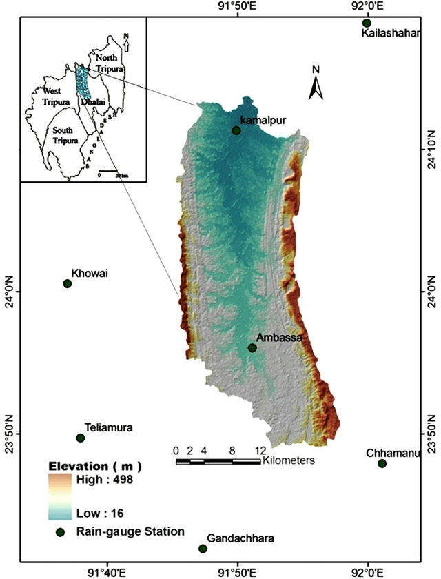
Figure 1. Location of the study area with Digital Elevation Model (DEM) and Rain-gauge stations.
Although the USLE model was developed for agricultural areas with slopes from 3% to 18%, it still widely applied in many countries, including India, for local scale studies and it is the most widely used model to estimate soil loss from watersheds [43]. Its successful use with or without modification in hilly and mountain regions was reported [23,25,38,44,45]. A set of experiments have been done to adopt this model in different geographical conditions in India, [42,46,47]. As this model is developed for erosion assessment at local scale, some modifications are necessary, to be applied at regional scale, because of lower information content of available data.
Generally, the USLE model defines annual soil loss (A) (t∙h−1∙y−1) as a product of six main factors: rainfall erosivity (R factor), soil erodibility (K factor), slope length (L factor), slope angle (S factor), land cover (C factor) and conservation practice (P factor). It is expressed by empirically derived Equation (1):
 (1)
(1)
The assessment of soil erosion at watershed level can be exercised in two ways—calculation of the potential soil loss (EP) (Equation (2)) and calculation of actual average annual soil loss (EA) (Equation (3)). Equations (2) and (3) indicates the method of estimating potential and actual soil loss:
 . (2)
. (2)
 (3)
(3)
3.1. Data Layers
3.1.1. Rain Erosivity (R) Factor
Soil erosion is closely related to rainfall through the combined effect of detachment by raindrops striking the soil surface and by the runoff [48]. According to USLE method, soil loss from the cultivated field is directly proportional to a rain storm parameter, if other factors remain constant. Rain-erosivity (R) is calculated as a product of storm kinetic energy (E) and the maximum 30 minutes rain fall intensity. This relationship [14] helps to quantify the impact of rain drop over a piece of land and the rate of runoff associated with the rain. But till now that kind of detailed meteorological data is not available for all the stations in the study area. Therefore, Equations (4) and (5) has been used for estimating annual and seasonal R factors [49] in Indian context.
 (4)
(4)
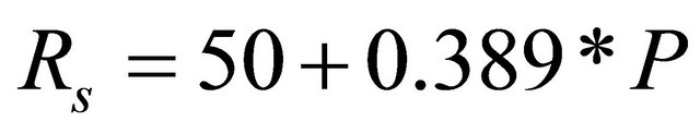 (5)
(5)
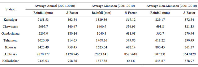
where, Ra is the annual R factor, Rs is the seasonal R factor and P is the Rainfall in mm. Rainfall data for 7 raingauge stations have so far been available for estimating the R factor, such as Kamalpur, Chawmanu, Gandachhara, Teliamura, Khowai, Ambassa and Kailashahar. Out of such seven rain-gauge stations only Kamalpur and Ambassa stations are situated within the river basin and the rest are outside the boundary of the basin. In this study, average annual rainfall erosivity (Ra) and seasonal rainfall erosivity (Rs) were calculated using rainfall data (Table 1) of these rain gauge stations for the years (2001 to 2010). R Factors data of these seven stations were imported into Arc GIS and interpolation method was used. In most of the available GIS software includes the inverse distance weighting (IDW), kriging, spline, polynomial trend and natural neighbor interpolation methods. In this study, IDW techniques available in Arc GIS 9.3 were used to interpolate a rainfall erosivity values. The IDW interpolation method was selected because the influence of rainfall erosivity is most significant at the measured point and decreases as distance increases away from the point.
3.1.2. Soil Erodibility Factor (K)
The soil erosivity factor (K) relates to the rate at which different soils erode. The K factor is rated on a scale from 0 to 1, with 0 indicating soils with the least susceptibility to erosion and whilst 1 indicates soils which are highly susceptible to soil erosion by water. The factor is defined as the rate of soil loss per rainfall erosion index unit as measured on a standard plot [50].
On the basis of the Geo-pedological map (Figure 2(a)) of the National Bureau of Soil Survey and Land Use Planning (NBSSLUP), Govt. of India Soil Erosivity Index factors (K) were evaluated by the soil erosivity Nomograph [14], using soil properties like sand, clay, silt, very fine sand, organic matter content in soils, structure type, and the permeability of soil (collected from the technical bulletin on soil series of Tripura and from the laboratory test of soil samples).
3.1.3. Topographic Erosivity Factor (LS)
The topographic factor consists of two sub-factors slope gradient and length of slope which significantly influence soil erosion by surface water movement.
Slope length factor (L) was calculated on the basis of the following method [51]:
 (6)
(6)
where L = slope length factor; λ = field slope length (m); m = dimensionless exponent that depends on slope steepness, being 0.5 for slopes exceeding 5%, 0.4 for 4% slopes and 0.3 for slopes less than 3%. The percent slope was determined for slope longer than 4 m on the basis of the following formulae [51]:
 (7)
(7)
 (8)
(8)
where, S = slope steepness factor and θ = slope angle in degree. The slope steepness factor is dimensionless.
In most of the cases it is found that LS value does not show the proper result of erosion below the slope length of 4 m.
3.1.4. Biological Erosivity Factor (CP)
C is the crop management factor and P is the erosion control practice or conservation factor. Most of the researchers have reported the use of these two factors as different factors when computing for USLE [5]. Some
Table 1. Average annual and seasonal rainfall (mm) and calculated R value for the stations considered for the study.
(a) 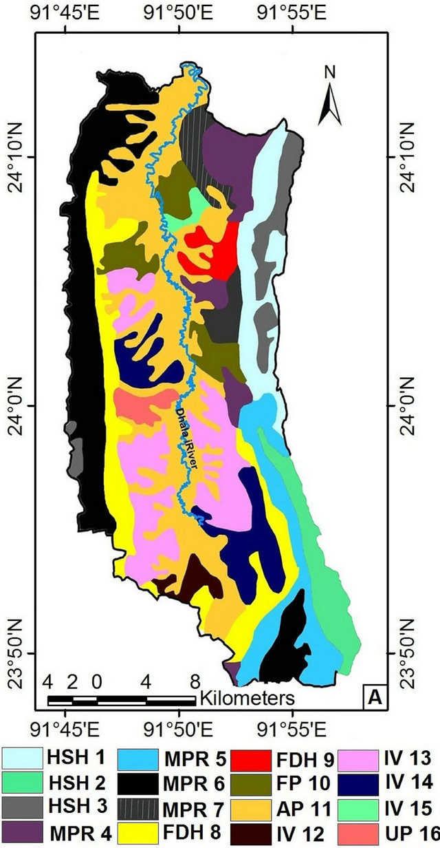 (b)
(b) 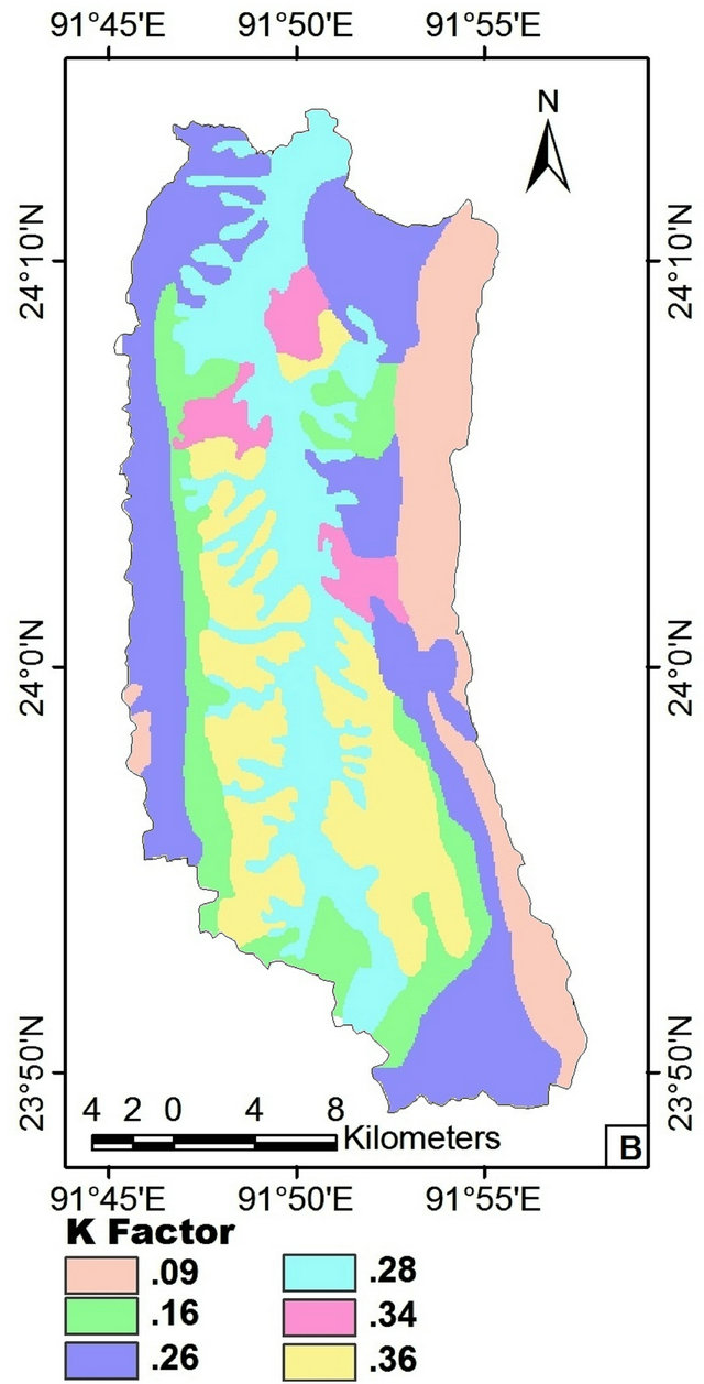
Figure 2. (a) Geo-pedological map of the study area; (b) Spatial distribution of K factor.
times, these two factors are also treated together as CP factor. For the present study, the combined CP factor has been used to estimate biological erosivity because majority of area under study is covered by different types of natural vegetation. Moreover, P factor can differ according to the farming practices and the level of conservation practice adopted particularly in the agricultural land. By interviewing the farmers during the field visit, it was found that soil conservation measures are not adopted in the area at significantly. As there is only a very small area has conservation practices in the study area, P factor values are assumed as 1 for the basin.
4. Results and Discussion
4.1. Rain Erosivity (R)
The annual average rainfall erosivity factor (Ra) was found to be in the range of 959.45 to 814.65 t∙h−1∙y−1. The highest value (1409.014 t∙h−1∙y−1) of annual R factor was observed in the year of 2010 in Ambassa station when the total annual rain fall was 3663.95 mm. The lowest value (615.49 t∙h−1∙y−1) was observed to be in the year of 2006 when the total rainfall was 1477.7 mm at Kamalpur station (Table 1). In present study area the annual R value gradually decreased towards north from Ambassa (Figure 3(a)). The average Monsoon and nonmonsoon R factor of these seven rain gauge stations is ranges from 688.08 to 567.12 and 270.44 to 378.97 t∙h−1∙y−1 respectively. The maximum value (852.5618 t∙h−1∙y−1) of average monsoon R factor was found at Ambassa station where the recorded average monsoonal (June-October) rainfall was 2063.14 mm. In case of nonmonsoon, the maximum value (378.97 t∙h−1∙y−1) was found at Kailashahar station where the recorded average monsoonal rainfall was 845.67 mm. So, there is a spatiotemporal variation in seasonal R factor. In the present study area, seasonal variations of R factors are shown in the iso-erodent maps of spatial distribution of average monsoon and non-monsoon R factors (Figures 3(b) and (c)).
4.2. Soil Erodibility (K)
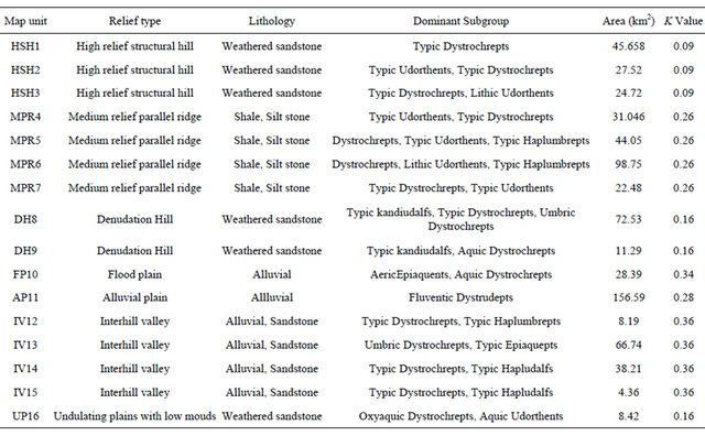
A detailed table has been prepared to show the relief type, lithology, dominant subgroups, area and the calculated K values associated with different soil types (Table 2). Soil type varies from one place to another on the basis of topographical and lithological characteristics. Different soil codes have been determined to designate different soil types on the basis of relief types (e.g. “H” stands for High relief, “SH” for Structural hill and so on).
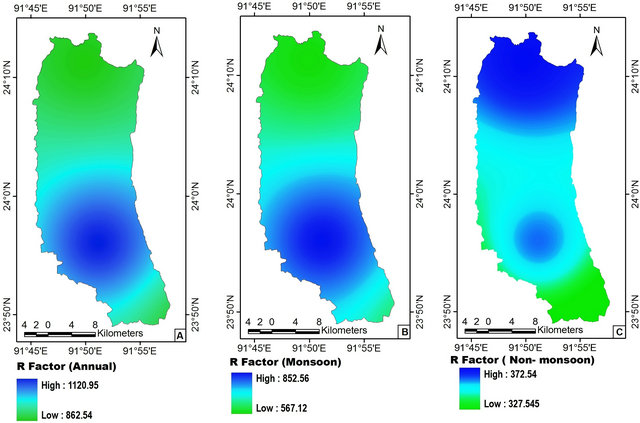
Figure 3. Spatial distribution of R factor (A for annual, B for monsoon and C for non-monsoon R factors).
Table 2. Geo-pedological index corresponding to Figure 2(a).
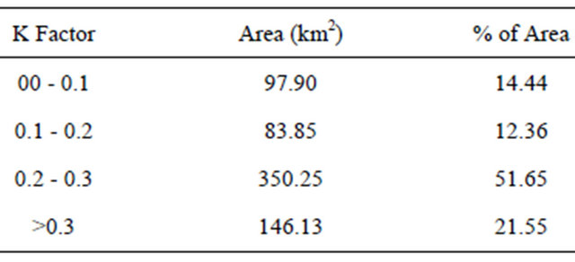
K values of different soil types have been estimated from the Nomograph (Wischmeier and Smith, 1978) of USLE. By plotting the K values in respect to different soil types, the soil erodibility map of the study area has been prepared (Figure 2(b)). The K factor map shows a maximum value of 0.36 with a mean of 0.24 and minimum value of 0.09. In high relief and Denudation hill areas, the K value is generally ranges from 0.09 to 0.16, but in low relief areas like alluvial plains, flood plains an inter-hill valley region, the K value is became high which is ranges from 0.28 to 0.036. The maximum K value (0.36) was found in interhill valley region Spatial distribution of K value has shown in Table 3. From the study it has been found that very less (<1) K factor was found in only 14.44% of the total area where Major portion (51.65) of the total basin was accounted for K values 0.2 to 0.3.
4.3. Topographic Erosivity (LS)
The LS factor in the present study area was found to be in the range of 0.82 to 53. The lowest values for the LS factor were mainly found along the river that flows towards north, because the slope values are very low. The higher (>20) LS factor values were found mainly in the east and west however, the very high LS values (>30) ware found in small areas particularly located in the northeastern Middle Western part (Figure 4) of the where the slope is generally high. From the study, it has been found that very low (<5) LS values ware found in 26.66% of the total area where only 2.73% (Table 4) of the study area was accounted for LS values more than 30. In gently sloping (mainly in flood plains) areas, the topographic factor ranges from 0.83 to 4.79. Moderately sloping area possess topographic factor between 5.08 and 9.76. High and very high topographic factors are noticed in the area of moderately steep to very steeply sloping landforms (mainly hill side slopes).
4.4. Biological Erosivity (CP)
The land cover type of the study area has prepared by classifying the satellite data along with intensive ground truth verification with the help of GPS. Five types of land cover/land-uses have been identified in the whole Dhalai river basin, viz., dense deciduous forest, moderately dense
Table 3. Spatial distribution of K factor in the study area.
forest, degraded forest, Agricultural land and water bodies. Land cover (Figure 5) information was thus available for the basin. The C factor values in the watershed vary from 0 to 0.39. The lower C factor values are seen in the east, west and southern part of the basin where majority of land is characterized by dense to moderately dense forest. However, the degraded forest and agricultural areas which occupy the middle and southern portion have high C factor values (Figure 5). Present study revealed that 63.95% of the total study area is under dense to moderately dense forest cover where C factor was reported 0.02 to 0.04 (Table 5).
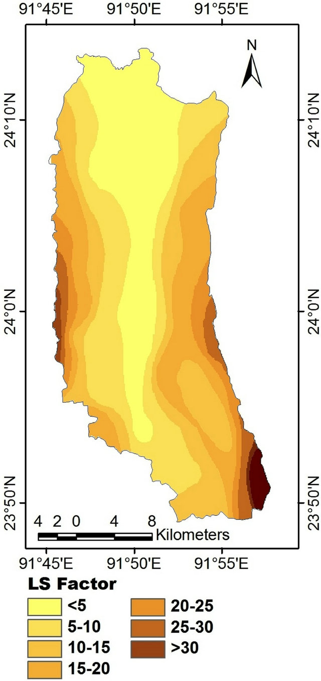
Figure 4. Spatial distribution of LS factor.
Table 4. Spatial distribution of LS factor in the study area.
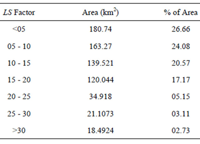

Figure 5. Land-use/land cover map of the study area.
Table 5. Assessment of C factor associated with different land-use/land cover.

The P factor values are determined according to the soil conservation techniques used in the study area. From the field survey no conservation techniques for controlling this excessive erosion were found. There are no data available for identifying soil conservation techniques in the study area. Because no conservation techniques were used in the study area, P factor value was set to 1 for the entire watershed area.
4.5. Potential and Actual Soil Loss
After completing data input procedure and preparation of the appropriate maps as data layers, they are multiplied in order to get an estimate of the potential and actual rate of soil erosion. Potential soil erosion expresses the inherent susceptibility of bare soil to erosion as it would be without any protective cover of vegetation. This way it provides information on the worst possible situation that might occur. In present study area, the low potential zone have found in flood plain region where as the high potential zone have found in hill sides steep slope areas (Figure 6). Actual soil erosion refers to present endangerment, taking into account contemporary land cover and management practices that modify the potential erosion.
In order to predict the annual average soil loss rate in the Dhalai river basin, all parameters of the USLE model are multiplied. Figure 7 represents the spatial distribution of actual annual average soil loss rate of the river basin. The maximum soil loss rate (836 t∙h−1∙y−1) occurs at the agricultural field and minimum soil loss rate is predicted to be 11 t∙h−1∙y−1) in dense forest cover area. The occurrence of soil erosion has a close relationship with the status of land use and the type of soil along with topographical characteristics such as slope length and steepness. The comparatively lower rate (<50 t∙h−1∙y−1) of erosion was found in western, eastern and southeastern parts of the basin where land-use/land-cover is mainly characterized by dense to moderately dense forest. The
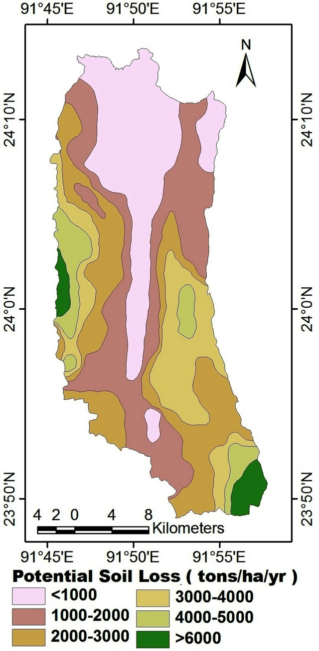
Figure 6. Spatial distribution of potential soil loss.
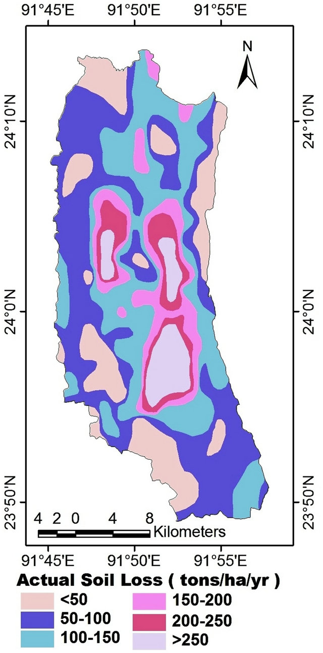
Figure 7. Spatial distribution of actual soil loss.
very high to severe rate (>200 t∙h−1∙y−1) of erosion was observed in middle part of the basin where maximum part of the land is under degraded forest or using for agriculture purpose and high value of K factor. In Dhalai river basin only 17.33% of the total land is under comparative low (<50 t∙h−1∙y−1) erosion zone (Table 6). Present study revealed that 48.16% of the total study area is experienced with the erosion rate >200 t∙h−1∙y−1.
Actual average annual soil erosion map has reclassified (Figure 8) on the basis of average rate of erosion in different sub watersheds in order to identify the most erosion prone sub-watersheds in the basin. The sub watersheds (SW) have been classified into three categories, where SW1, SW2, SW3, SW4, SW9, SW10, SW11, SW12, SW13 are falling in relatively low (<100 tons/ha/ yr) zone and SW5, SW6, SW7, SW8, SW17, SW18, SW19, SW22 are in relatively moderate (100 - 200 tons/ha/yr) zone and SW14, SW15, SW16, SW20, SW21, SW23 are falling in relatively high(>200 t∙h−1∙y−1) erosion zone. The maximum and minimum average annual rates of erosion have also been calculated of each sub watersheds which has shown in Table 7. To understand the variation of the rate of erosion, standard deviation of each sub watershed has also been calculated. The maximum (246.88 t∙h−1∙y−1) standard deviation has found in SW20, mainly because of variation of land cover and soil
Table 6. Spatial distribution of actual soil loss.
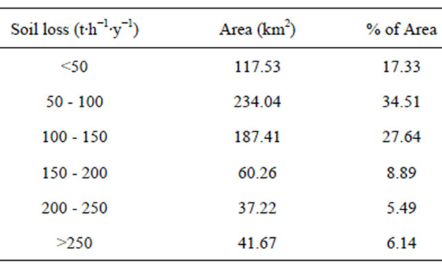
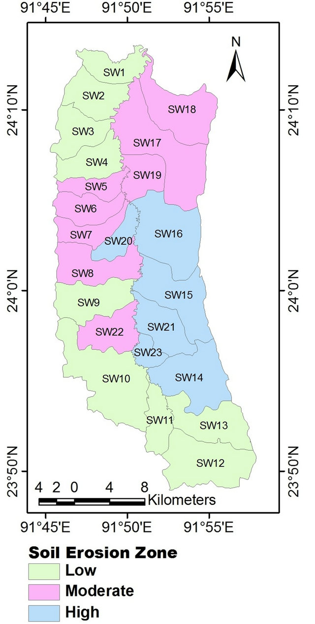
Figure 8. Soil erosion priority Zonation at sub-watersheds level.
type and minimum (29.53 t∙h−1∙y−1) standard deviation has found in SW4.
To understand the relative importance of different factors, the average parametric value of all factors of all sub watersheds have been estimated and shown in Table 7. From this table, it is clear that the rain erosivity (R) factor is varying in some extends and ranges from 868.62 to 1116.51. The maximum value was found in Lal chhara (SW23) sub-watershed and the minimum value was found in Joysindhubari (SW1) sub-watershed.
Average K value of different sub-watershed is also not varying in grate extends and it ranges from 0.2 (SW3) to 0.33 (SW22). Average Topographic erosivity (LS) factor
Table 7. Assessment of average parametric values of all parameters and calculation of maximum, minimum and variations of erosion rate in different sub-watersheds and categories them on the basis of average rate of erosion.
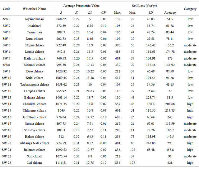
of different sub-watershed in this study area is varying from 5 to 24.63. The maximum value was observed in Lampha chhara (SW12) sub-watershed where it is characterized by upper catchment of the basin. CP factor of different sub-watershed also ranges from 0.04 to 0.11. The LS and CP factors are varying in some extend because some sub-watershed are falling in Upper catchment which are showing high slope and dense to moderately dense forest cover and some sub-watersheds in lower and middle portion of the basin shows comparatively low slope and degraded to agricultural land areas.
5. Conclusions
By assuming no support practice in the study area (P = 1), the annual soil losses (A in t∙h−1∙y−1) with respect to the different land-use/land-cover types of the region were estimated as a product of R, K, LS, and C layers. In terms of the land uses, especially the agricultural land and degraded forest cover areas were found to be more susceptible to the soil losses by water erosion than dense forest, moderately dense forest cover areas. The rate of soil erosion has been changed mainly due to the changing of landuse pattern since the rain fall has changed only with slightly. Moreover, rate of soil loss from different sub watersheds is mainly dependent on LS and CP factors. Researchers [52-55] concluded that traditional USLE method can be used for identifying the areas prone to high level erosion risks. In present study, the result also shows that the USLE is very helpful for estimating the rate of erosion as well as to identify the erosion prone areas in basin. Estimation of predicted amount of soil loss from the different sub-watershed and its spatial distribution can be helpful for suitable management and sustainable land use for the present study area.
However, there is a need to have direct field measurements of soil erosion in the watershed to confirm and validate the results of USLE prediction. Therefore, future works are required for monitoring of sediment load in rivers and measurement of sediment deposition in river and other water bodies that exist in the watershed.
6. Acknowledgements
The present paper is a part of the University Grants Commission (UGC), India funded major project on “A Study of Landslides through hazard zonation, risk analysis and preparation of landslide inventory of Dhalai district in the state of Tripura using RS and GIS techniques”. The authors are grateful to the learned reviewers for their suggestions given for upgrading the paper.
REFERENCES
- S. D. Angima, D. E. Stott, M. K. O’Neill, C. K. Ong and G. A. Weesies, “Soil Erosion Prediction Using RUSLE for Central Kenyan Highland Conditions,” Agriculture, Ecosystems & Environment, Vol. 97, No. 1-3, 2003, pp. 295-308. doi:10.1016/S0167-8809(03)00011-2
- S. Nanna, “A Geo-Information Theoretical Approach to Inductive Erosion Modeling Based on Terrain Mapping Units,” Ph.D. Thesis, Wageningen Agricultural University, Wageningen, 1996.
- Y. S. Elirehema, “Soil Water Erosion Modeling in Selected Watersheds in Southern Spain,” IFA, ITC, Enschede, 2001.
- A. Pandey, A. Mathur, S. K. Mishra and B. C. Mal, “Soil Erosion Modeling of a Himalayan Watershed Using RS and GIS,” Environmental Earth Sciences, Vol. 59, No. 2, 2009, pp. 399-410. doi:10.1007/s12665-009-0038-0
- K. C. Bahadur, “Mapping Soil Erosion Susceptibility Using Remote Sensing and GIS: A Case of the Upper Nam Wa Watershed, Nan Province, Thailand,” Environmental Geology, Vol. 57, 2008, pp. 695-705. doi:10.1007/s00254-008-1348-3
- G. Wang, G. Gertner, S. Fang and A. B. Anderson, “Mapping Multiple Variables for Predicting Soil Loss by Geostatistical Methods with TM Images and a Slope Map,” Photogrammetric Engineering & Remote Sensing, Vol. 69, 2003, pp. 889-898.
- R. Lal, “Deforestation and Land Use Effects on Soil Degradation and Rehabilitation in Western Nigeria. III. Runoff, Soil Erosion and Nutrient Loss,” Land Degradation & Development, Vol. 7, No. 2, 1996, pp. 99-119. doi:10.1002/(SICI)1099-145X(199606)7:2<99::AID-LDR220>3.0.CO;2-F
- C. W. Rose and R. C. Dalal, “Erosion and Runoff of Nitrogen,” In: J. R. Wilson, Ed., Advances in Nitrogen Cycling in Agricultural Ecosystems, CAB International, Wallingford, 1988, pp. 212-235.
- D. Ouyang and J. Bartholic, “Predicting Sediment Delivery Ratio in Saginaw Bay Watershed,” Proceedings of the 22nd National Association of Environmental Professionals Conference, Orlando, 19-23 May 1997, pp. 659-671.
- V.V. Dhruvanarayana and R. Babu, “Estimation of Soil Loss in India,” Journal of Irrigation and Drainage Engineering, Vol. 109, No. 4, 1983, pp. 419-433. doi:10.1061/(ASCE)0733-9437(1983)109:4(419)
- V. Prasannakumar, R. Shiny, N. Geetha and H. Vijith, “Spatial Prediction of Soil Erosion Risk by Remote Sensing, GIS and RUSLE Approach: A Case Study of Siruvani River Watershed in Attapady Valley, Kerala, India,” Environmental Earth Sciences, Vol. 64, No. 4, 2011, pp. 965-972. doi:10.1007/s12665-011-0913-3
- M. Kouli, P. Soupios and F. Vallianatos, “Soil Erosion Prediction Using the Revised Universal Soil Loss Equation (RUSLE) in a GIS Framework, Chania, Northwestern Crete, Greece,” Environmental Geology, Vol. 57, No. 3, 2009, pp. 483-497. doi:10.1007/s00254-008-1318-9
- W. H. Wischmeier and D. D. Smith, “Predicting RainfallErosion Losses from Cropland East of the Rocky Mountains, Guide for Selection of Practices for Soil and Water Conservation,” Agriculture Handbooks, US Government Print Office, Washington, 1965.
- W. H. Wischmeier and D. D. Smith, “Predicting Rainfall Erosion Loss: A Guide to Conservation Planning,” Agricultural Handbook, No. 537, US Department of Agriculture, Agricultural Research Service, Washington, 1978.
- R. Lal, “Soil Degradation by Erosion,” Land Degradation & Development, Vol. 12, No. 6, 2001, pp. 519-539. doi:10.1002/ldr.472
- K. G. Renard, G. R. Foster, G. A. Weesies and J. P. Porter, “RUSLE, Revised Universal Soil Loss Equation,” Journal of Soil and Water Conservation, Vol. 46, No. 1, 1991, pp. 30-33.
- J. O. Onyando, P. Kisoyan and M. C. Chemelil, “Estimation of Potential Soil Erosion for River Perkerra Catchment in Kenya,” Water Resources Management, Vol. 19, No. 2, 2005, pp.133-143. doi:10.1007/s11269-005-2706-5
- G. R. Foster, L. J. Lane, J. D. Nowlin, J. M. Laflen and R. A. Young (1980) “A model to Estimate Sediment Yield from Field-Sized Areas: Development of Model,” In: W. G. Knisel, Ed., CREAMS: A Field Scale Model for Chemicals, Runoff, and Erosion from Agricultural Management Systems, US Department of Agriculture, Vol. 26, 1980, pp. 36-64.
- M. A. Nearing, G. R. Foster, L. J. Lane and S. C. Finkner, “A Processbased Soil Erosion Model for USDA-Water Erosion Prediction Project Technology,” Tasea, Vol. 32, No. 5, 1989, pp. 1587-1593.
- R. P. C. Morgan, J. N. Quinton, R. E. Smith, G. Govers, J. W. A. Poesen, K. Auerswald, G. Chisci, D. Torri and M. E. Styczen, “The European Soil Erosion Model (EUROSEM): A Dynamic Approach for Predicting Sediment Transport from Fields and Small Catchments,” Earth Surface Processes and Landforms, Vol. 23, No. 6, 1998, pp. 527-544. doi:10.1002/(SICI)1096-9837(199806)23:6<527::AID-ESP868>3.0.CO;2-5
- J. Schmidt, M. V. Werner and A. Michael, “Application of the EROSION 3D Model to the Catsop Watershed, The Netherlands,” Catena, Vol. 37, No. 3-4, 1999, pp. 449-456. doi:10.1016/S0341-8162(99)00032-6
- R, Lal and W. H. Blum, “Methods for Assessment of Soil Degradation,” In: Advances in Soil Science, CRC Press, Boca Raton, 1997, p. 558.
- A. A. Millward and J. E. Mersey, “Adapting the RUSLE to Model Soil Erosion Potential in a Mountainous Tropical Watershed,” Catena, Vol. 38, No. 2, 1999, pp. 109- 129. doi:10.1016/S0341-8162(99)00067-3
- T. Chen, R. Niu, P. Li, L. Zhang and B. Du, “Regional Soil Erosion Risk Mapping Using RUSLE, GIS, and Remote Sensing: A Case Study in Miyun Watershed,” Environmental Earth Sciences, Vol. 63, No. 3, 2010, pp. 533-541.
- J. B. Kim, P. Saunders and J. T. Finn, “Rapid Assessment of Soil Erosion in the Rio Lempa Basin, Central America, Using the Universal Soil Loss Equation and Geographic Information Systems,” Journal of Environmental Management, Vol. 36, No. 6, 2005, pp. 872-885. doi:10.1007/s00267-002-0065-z
- A. Martin, J. Gunter and J. Regens, “Estimating Erosion in a Riverine Watershed, Bayou Liberty-Tchefuncta River in Louisiana,” Environmental Science and Pollution Research, Vol. 10, No. 4, 2003, pp. 245-250. doi:10.1065/espr2003.05.153
- A. U. Ozcan, G. Erpul, M. Basaran and H. E. Erdogan, “Use of USLE/GIS Technology Integrated with Geostatistics to Assess Soil Erosion Risk in Different Land Uses of Indagi Mountain Pass-Cankırı,” Environmental Geology, Vol. 53, No. 8, 2008, pp. 1731-1741. doi:10.1007/s00254-007-0779-6
- E. H. Erdogan, G. Erpul and I. Bayramin, “Use of USLE/ GIS Methodology for Predicting Soil Loss in a Semiarid Agricultural Watershed,” Environmental Monitoring and Assessment, Vol. 131, No. 1-3, 2007, pp. 153-161. doi:10.1007/s10661-006-9464-6
- R. Bhattarai and D. Dutta, “Estimation of Soil Erosion and Sediment Yield Using GIS at Catchment Scale,” Water Resources Management, Vol. 21, No. 10, 2007, pp. 1635-1647. doi:10.1007/s11269-006-9118-z
- A. Demirci and A. Karaburun, “Estimation of Soil Erosion Using RUSLE in a GIS Framework: A Case Study in the Buyukcekmece Lake Watershed, Northwest Turkey,” Environmental Earth Sciences, Vol. 66, No. 3, 2011, pp. 903-913. doi:10.1007/s12665-011-1300-9
- J. Van der Knijff, R. J. A. Jones and L. Montanarella, “Soil Erosion Risk Assessment in Italy,” European Soil Bureau, Joint Research Center of European Commission, EUR 19022EN, 2000.
- P. Veljko, L. Zivotic, R. Kadovic, A. Dordevic, D. Jaramaz, V. Mrvic and M. Todorovic, “Spatial Modelling of Soil Erosion Potential in a Mountainous Watershed of South-Eastern Serbia,” Environmental Earth Sciences, Vol. 68, No. 1, 2013, pp. 115-128. doi:10.1007/s12665-012-1720-1
- L. Mitas and H. Mitasova, “Distributed Soil Erosion Simulation for Effective Erosion Prevention,” Water Resources Research, Vol. 34, No. 3, 1998, pp. 505-516. doi:10.1029/97WR03347
- J. R. Williams and H. D. Berndt, “Sediment Yield Computed with Universal Equation,” Journal of the Hydraulics Division, Vol. 98, No. 12, 1972, pp. 2087-2098.
- M. L. Griffin, D. B. Beasley, J. J. Fletcher and G. R. Foster, “Estimating Soil Loss on Topographically Non-Uniform Field and Farm Units,” Journal of Soil and Water Conservation, Vol. 43, No. 4, 1988, pp. 326-331.
- S. K. Jain, S. Kumar and J. Varghese, “Estimation of Soil Erosion for a Himalayan Watershed Using GIS Technique,” Water Resources Management, Vol. 15, No. 1, 2001, pp. 41-54. doi:10.1023/A:1012246029263
- S. M. J. Baba and K. W. Yusof, “Modelling Soil Erosion in Tropical Environments Using Remote Sensing and Geographical Information Systems,” Journal of Hydrology Science, Vol. 46, No. 1, 2001, pp. 191-198.
- P. P. Dabral, N. Baithuri and A. Pandey, “Soil Erosion Assessment in a Hilly Catchment of North Eastern India Using USLE, GIS and Remote Sensing,” Water Resources Management, Vol. 22, No. 12, 2008, pp. 1783- 1798. doi:10.1007/s11269-008-9253-9
- J. C. Sharma, J. Prasad, S. K. Saha and L. M. Pande, “Watershed Prioritization Based on Sediment Yield Index in Eastern Part of Don Valley Using RS and GIS,” Indian Journal of Soil Conservation, Vol. 29, No. 1, 2001, pp. 7- 13.
- M. A. Khan, V. P. Gupta and P. C. Moharana, “Watershed Prioritization Using Remote Sensing and Geographical Information System: A Case Study from Guhiya,” India Journal of Arid Environments, Vol. 49, No. 3, 2001, pp. 465-475. doi:10.1006/jare.2001.0797
- R. K. Saxena, K. S. Verma, G. R. Chary, R. Srivastava and A. K. Barthwal, “IRS-1C Data Application in Watershed Characterization and Management,” International Journal of Remote Sensing, Vol. 21, No. 17, 2000, pp. 3197-3208. doi:10.1080/014311600750019822
- R. S. Chaudhary and P. D. Sharma, “Erosion Hazard Assessment and Treatment Prioritization of Giri River Catchment, North Western Himalayas,” Indian Journal of Soil Conservation, Vol. 26, No. 1, 1998, pp. 6-11.
- V. V. Rao, A. K. Chakravarty and U. Sharma, “Watershed Prioritization Based on Sediment Yield Modeling and IRS-1A LISS Data,” Asian-Pacific Remote Sensing Journal, Vol. 6, No. 2, 1994, pp. 59-65.
- A. Irvem, F. Topaloglu and V. Uygur, “Estimating Spatial Distribution of Soil Loss over Seyhan River Basin in Turkey,” Journal of Hydrology, Vol. 336, No. 1-2, 2007, pp. 30-37. doi:10.1016/j.jhydrol.2006.12.009
- P. Zhou, O. Luukkanen, T. Tokola and J. Nieminen, “Effect of Vegetation Cover on Soil Erosion in a Mountainous Watershed,” Catena, Vol. 75, No. 3, 2008, pp. 319- 325. doi:10.1016/j.catena.2008.07.010
- S. Biswas, S. Sudhakar and V. R. Desai, “Prioritization of Subwatersheds Based on Morphometric Analysis of Drainage Basina Remote Sensing and GIS Approach,” Photonirvachak, Vol. 27, 1999, pp. 155-166.
- S. K. Jain and M. K. Goel, “Assessing the Vulnerability to Soil Erosion of the Ukai Dam Catchments Using Remote Sensing and GIS,” Hydrological Sciences, Vol. 47, No. 2, 2002, pp. 31-40. doi:10.1080/02626660209492905
- M. M. Mkhonta, “Use of Remote Sensing and Geographical Information System (GIS) on Soil Erosion Assessment in the Gwayimane and Mahhuku Catchment Areas with Special Attention on Soil Erodobility (K-Factor),” ITC, Enschede, 2000.
- G. Singh, V. V. Rambabu and S. Chandra, “Soil Loss Prediction Research in India,” ICAR Bullet, T12/D9, CS WCTRI, Dehradun, 1981.
- P. Mhangara, V. Kakembo and K. J. Lim, “Soil Erosion Risk Assessment of the Keiskamma Catchment, South Africa Using GIS and Remote Sensing,” Environmental Earth Sciences, Vol. 65, No. 7, 2012, pp. 2087-2102. doi:10.1007/s12665-011-1190-x
- D. K. McCool, G. R. Foster, C. K. Mutchler and L. D. Meyer, “Revised Slope Steepness Factor for the Universal Soil Loss Equation,” Transactions of the ASAE, Vol. 30, No. 5, 1987, pp. 1387-1396.
- B. Mitra, H. D. Scott, J. C. Dixon and J. M. McKimmey, “Applications of Fuzzy Logic to the Prediction of Soil Erosion in a Large Watershed,” Geoderma, Vol. 86, No. 3-4, 1998, pp. 183-209. doi:10.1016/S0016-7061(98)00050-0
- T. R. N. Ahamed, G. K. Rao and J. S. R. Murthy, “Fuzzy Class Membership Approach to Soil Erosion Modeling,” Agricultural Systems, Vol. 63, No. 2, 2000, pp. 97-110. doi:10.1016/S0308-521X(99)00066-9
- G. Metternicht, S. Gonzales and FUERO, “Foundation of a Fuzzy Exploratory Model for Soil Erosion Hazard Predict,” Environmental Modelling & Software, Vol. 20, No. 6, 2005, pp. 715-728. doi:10.1016/j.envsoft.2004.03.015
- A. H. Sheikh, S. Palria and A. Alam, “Integration of GIS and Universal Soil Loss Equation (USLE) for Soil Loss Estimation in a Himalayan Watershed,” Recent Research in Science and Technology, Vol. 3, No. 3, 2011, pp. 51- 57.
NOTES
*Corresponding author.