Journal of Flow Control, Measurement & Visualization
Vol. 1 No. 3 (2013) , Article ID: 37594 , 8 pages DOI:10.4236/jfcmv.2013.13011
Evaluation of Flight Trajectory and Unsteady Fluid Forces on Kicked Non-Spinning Soccer Ball by Digital Image Analysis
1Visualization Research Center, Niigata University, Ikarashi, Nishi-ku, Niigata, Japan
2Institute of Health and Sports Sciences, Tsukuba University, Tsukuba, Ibaraki, Japan
Email: yamagata@eng.niigata-u.ac.jp
Copyright © 2013 Takayuki Yamagata et al. This is an open access article distributed under the Creative Commons Attribution License, which permits unrestricted use, distribution, and reproduction in any medium, provided the original work is properly cited.
Received May 13, 2013; revised July 17, 2013; accepted August 5, 2013
Keywords: Non-Spinning Soccer Ball; Fluid Force; Flight Trajectory; Measurement; Stereo Image Analysis
ABSTRACT
This paper describes the experimental method for evaluating the flight trajectory and the aerodynamic performance of a kicked non-spinning soccer ball. The flight trajectory measurement is carried out using the digital image analysis. A centroid method and a template matching method are tested for the flight trajectory analysis using the artificial images generated by the data of a free-fall experiment. The drag coefficient obtained by the centroid method is better suited for the sports ball experiment than that by the template matching method, which is due to the robustness of the centroid method to the non-uniform illumination. Then, the flight trajectory analysis is introduced to a kicked experiment for a non-spinning soccer ball. The experimental result obtained from the stereo observation indicates that the S-shaped variation is found in the three-dimensional flight trajectory and in the side force coefficient during the flight of the nonspinning soccer ball.
1. Introduction
Aerodynamic properties of a flying sports ball have been a topic of great interests in the field of sports science and engineering. For example, the effects of dimple shape and the spin on the flying distance of golf ball were studied [1,2] and the influence of seams and rotation on the aerodynamic properties were investigated for baseball [3, 4]. Furthermore, the aerodynamic characteristics were evaluated for soccer balls [5-12]. In the past, the aerodynamic properties of sports ball were studied by wind-tunnel experiments, which allow the evaluation of time-averaged statistics of the sports ball in high accuracy [7,12]. Although such wind tunnel studies provide fundamental information on the aerodynamic properties acting on the sports balls, it is difficult to evaluate the unsteady aerodynamic properties of kicked soccer ball. Furthermore, the initial ball speed and the flight trajectory of a kicked soccer ball are affected by the ball deformation in the kick. Therefore, there is a difficulty in evaluating the flight trajectories and unsteady fluid forces on a kicked soccer ball by wind-tunnel experiment.
One approach to evaluate unsteady aerodynamic properties of a soccer ball is a flight trajectory analysis combined with imaging techniques. In the past, the flight trajectory of a soccer ball was observed by a high-speed camera, and the two-dimensional flight trajectory of the soccer ball was examined [5,8,10]. These experiments allow the evaluation of unsteady fluid forces acting on the ball, but it is limited to in-plane components of observation. On the other hand, three-dimensional trajectory measurement was carried out for the flight trajectory analysis of a spinning soccer ball [6]. In this study, three-dimensional flight trajectory and rotation speed were measured with high accuracy, though 13 cameras were used for the measurement.
Since the FIFA World Cup in 2006, the panel design of the soccer ball has been changed and the surface of the ball became smoother than previous one. Then, the irregular flight trajectories such as curves, falls, or unsteady movements were observed more frequently than before. These changes in the flight trajectory of a soccer ball are called knuckle effects, and the aerodynamic performance has been studied in wind tunnel [7,12]. The experimental studies suggest the transition of the flow around a soccer ball from subcritical to supercritical at lower Reynolds number than that of the smooth sphere [7]. However, the physical mechanism of unsteadiness of a non-spinning soccer ball has not been fully understood due to the limitation of the wind tunnel studies, where the ball has to be fixed. In order to understand the knuckle effects more in detail, three-dimensional flight trajectory measurement has to be carried out for the kicked non-spinning soccer ball.
In recent years, high-speed observation of the flight trajectory combined with the digital image analysis has been studied and applied to the experimental fluid mechanics [13-17]. These measurements allow the evaluation of the in-plane fluid forces of a sphere in water entry by image analysis, where the centroid method [14] and the template matching method [16,17] are used for the flight trajectory analysis.
In the present study, three-dimensional flight trajectory analysis is developed for evaluating the aerodynamic properties of a non-spinning soccer ball. In the analysis, the centroid method and the template matching method are tested for evaluating the flight trajectory and the unsteady fluid forces, using artificial images combined with free-fall experiment. Then, the three-dimensional flight trajectory and the aerodynamic performance of the kicked non-spinning soccer ball are studied by the stereo observation.
2. Experimental Methods
2.1. Flight Trajectory Analysis
Flight trajectories of a soccer ball were measured by analyzing the sequential images taken from high-speed cameras. The determination of the center of the flying soccer ball is made by a centroid method and a template matching method. In the centroid method, the edge of the ball is determined from the steepest gradient of the intensity distribution, and then the ball center is evaluated in subpixel accuracy. Note that the intensity distribution inside the ball is considered uniform in order to remove the noise. In the template matching method, the ball center is determined by the cross-correlation calculation in subpixel accuracy [18], which is commonly used in the velocity measurement by particle image velocimetry. Note that the template image for detecting the ball center was generated artificially by computer graphics. It is assumed that the intensity distribution of the template image is approximated by the Gaussian distribution [19], and the intensity distribution is expressed by modifying the coefficients of the Gaussian distribution to fit with the experimental observation of the falling ball. The purpose of introducing the artificial image to the flight trajectory analysis is to minimize the influence of the image noise.
Time histories of fluid forces were evaluated from the flight trajectory analysis of the flying soccer ball. Since time intervals between successive images are small enough, the local velocity of the ball was calculated from the displacement of the ball center using the central difference method:
 (1)
(1)
where U is the ball velocity vector, X is the position vector of the ball center, t is the time, Δt is the time interval. The time interval was selected to keep the pixel displacement in the image larger than 20 pixels, which is roughly equivalent to the diameter of the soccer ball. Figure 1(a) shows an example of the velocity analysis of the flying soccer ball, showing the variations of ball position x and the ball velocity u with respect to the time t. In order to remove the noise, the moving average is incorporated into the analysis, which averages the instantaneous position data sampled at 10 data upstream and 10 data downstream of the target ball. Figure 1(a) shows the velocity of the ball with and without the averaging procedure. Then, the acceleration of the ball a was calculated by using the instantaneous velocities.
 (2)
(2)
The moving average is introduced into the acceleration analysis, too. Figure 1(b) shows the acceleration of the
 (a)
(a) (b)
(b)
Figure 1. Example of flight trajectory analysis. (a) Variations of ball position and velocity; (b) Variations of ball acceleration.
ball with and without the moving average. The averaged acceleration is much smoother than the instantaneous acceleration derived from Equations (1) and (2) without moving average. Note that the moving average is effective to reduce the random error in the instantaneous measurement of velocity and acceleration, while it deteriorates the spatial resolution of measurement. Therefore, the highly time-resolved measurement of flying ball position is essential to evaluate the velocity and the acceleration accurately.
The fluid force vector F acting on the soccer ball is calculated from the averaged acceleration, as follows:
 (3)
(3)
where m is the weight of the ball. The fluid forces acting on the ball are defined in Figure 2. The drag FD is defined by the force along the ball velocity U, the lift FL is perpendicular to the ball velocity, and the side force FS is perpendicular to the drag and lift forces. Then, the fluid force coefficients Cd, Cl, Cs are evaluated in non-dimensional form as follows:
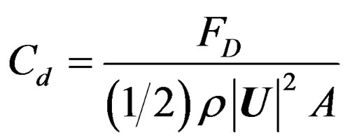 (4)
(4)
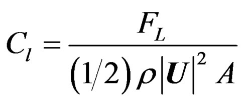 (5)
(5)
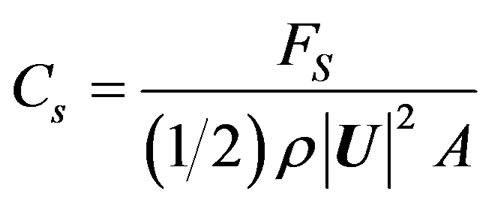 (6)
(6)
where ρ is the density of air, |U| is the magnitude of the local ball velocity, A is the projected area of the ball.
2.2. Free-Fall Experiment
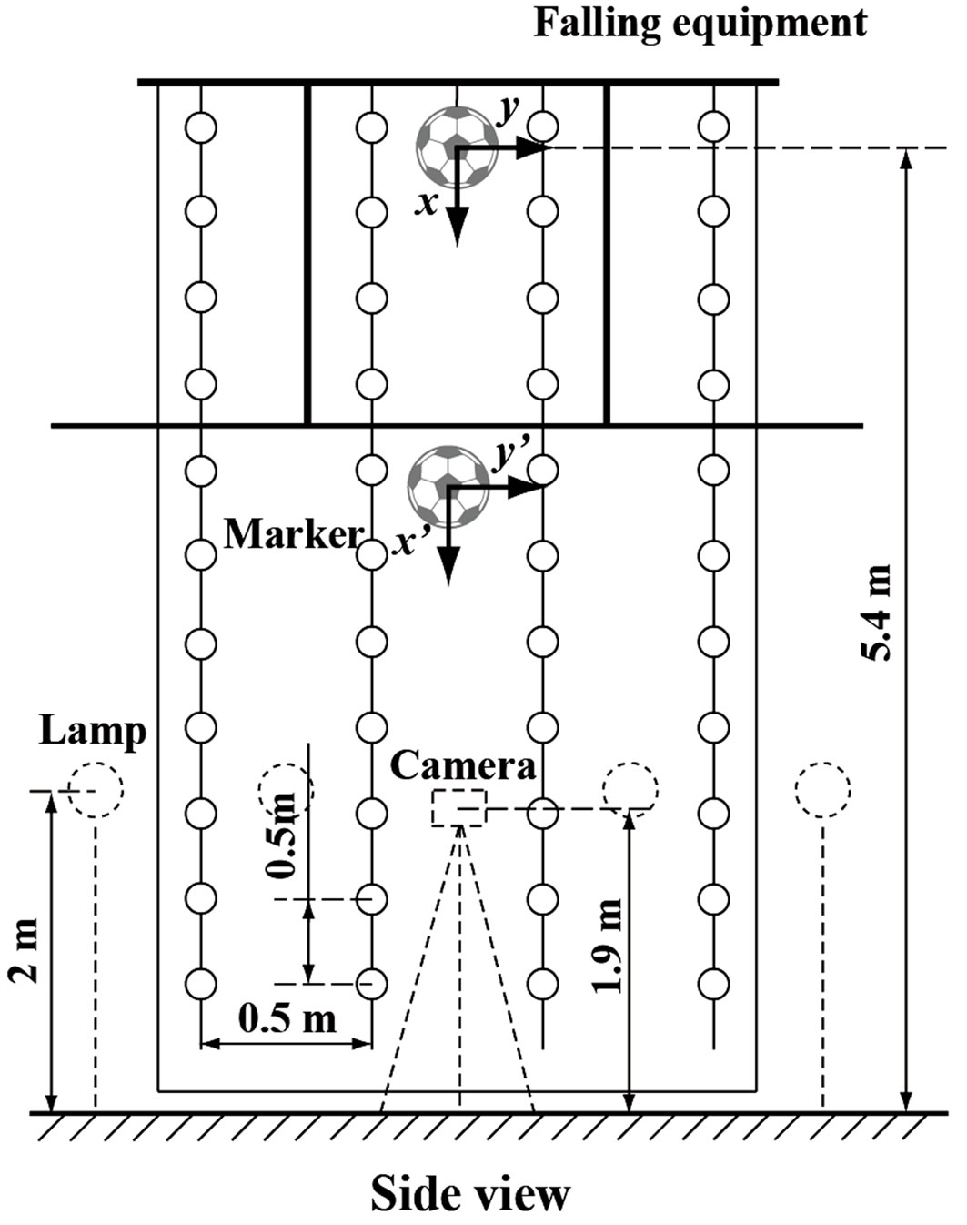
Figure 3 shows a schematic diagram of the experimental apparatus for the free-fall experiment. Figures 3(a) and (b) show the front and top views of the experimental apparatus, respectively. A soccer ball was dropped from the falling equipment located at 5.4 m in height from the floor. The soccer ball used in this study is shown in Figure 4, which is the official ball for the Beijing 2008 Olympic Games (Adidas teamgeist II), having a diameter of 220 mm and a weight 170 g. Note that the soccer ball has 14 panels on the surface.
The soccer ball was set on the falling equipment supported by a thin string. The start of the falling was made by cutting the string, which allows the free fall of the ball without rotation. A flight trajectory of the falling soccer ball was imaged by a high-speed CMOS camera, which was placed at 11.3 m in horizontal distance apart from the ball and at x = 3.5 m (1.9 m from the floor).
Sequential images of the falling soccer ball were recorded at the frame rate of 250 frames/sec. The spatial resolution of the image is 1280 × 1024 pixels with 8 bits. In order to remove the influence of lens distortion, the

Figure 2. Forces acting on a soccer ball.
 (a)
(a)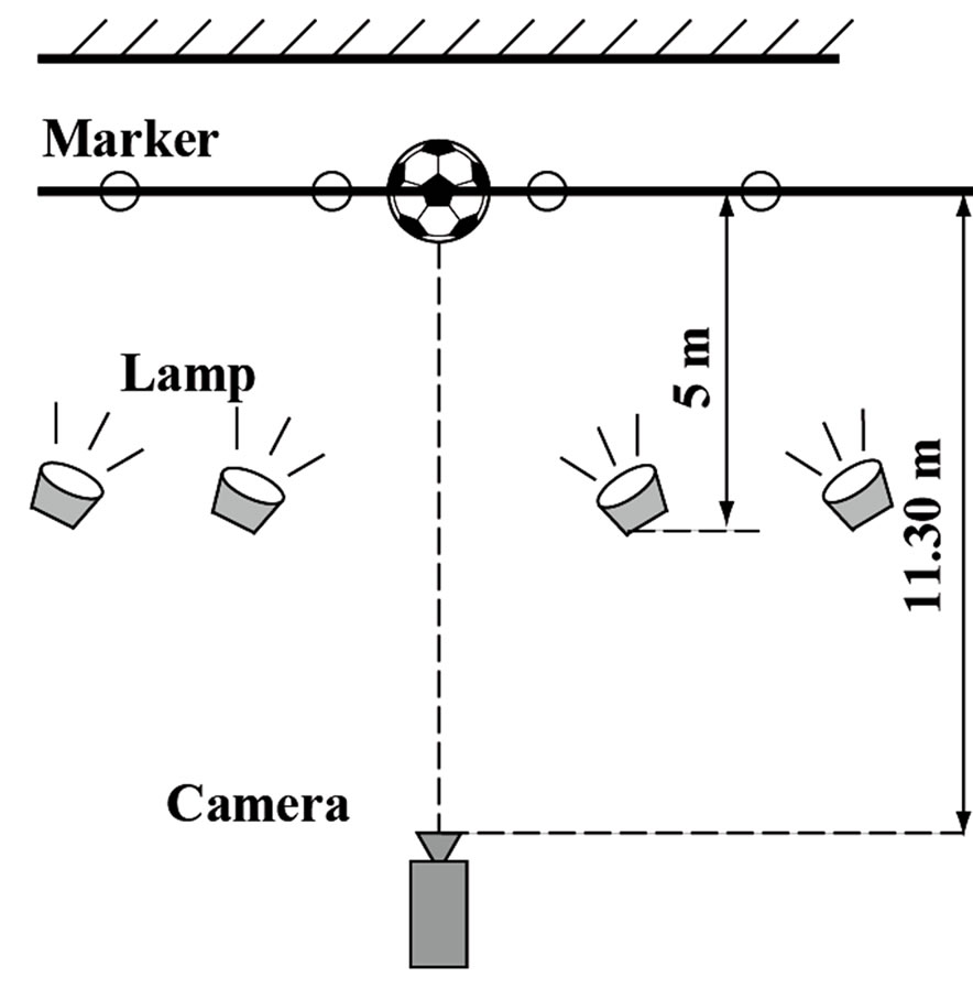 (b)
(b)
Figure 3. Experimental layout for free-fall test. (a) Front view; (b) Top view.
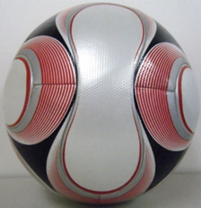
Figure 4. Soccer ball.
image deformation compensation was applied to the recorded images. The calibration was made against the markers placed at constant interval of 500 mm in the plane of the falling ball. The falling ball is illuminated by four halogen lamps placed at 5 m away from the ball and at x = 3.4 m (2 m from the floor).
2.3. Generation of Artificial Image
The artificial image of a falling ball was generated by the computer program based on Open GL (Open Graphics Library). The non-uniform intensity distribution on the ball is expressed by modifying the position of the light source and parameters of ambience, diffusion, and light direction in the program to fit with the experimental observation of the falling ball. It should be noted that the present artificial images are generated on the condition that the ball falls in gravitational direction without any fluid forces of air. The ball velocity U is expressed by the following equation
 (7)
(7)
where g is the gravitational acceleration. The artificial image allows the evaluation of the influence of light intensity distribution on the measurement accuracy of flight trajectory and the fluid forces.
2.4. Kicked Non-Spinning-Ball Experiment
Figure 5 shows a schematic diagram of the experimental layout for kicked non-spinning soccer ball. The experiment was conducted in the gymnasium in order to avoid the influence of wind. The three-dimensional position of the ball was determined from two synchronous CMOS cameras, which were located in the side view and in the front view of the flight trajectory. The two cameras are operated at 250 Hz with the camera lenses of focal length 16 mm and aperture 1.4. The observation volume was set as 10 × 2 × 4 m3 (x × y × z) and the focal plane was 12.5 m away from the kicker. Six halogen lamps were placed on the camera side of the flying soccer ball, as seen in Figure 5, to acquire the sequential ball images.
Stereo camera calibrations were done by locating the
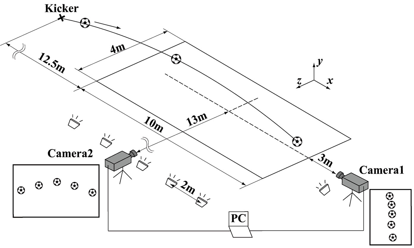
Figure 5. Experimental layout for non-spinning soccer ball.
poles of 2 m in length with the markers of 5 cm in diameter. The markers are placed at every 0.5 m intervals along the pole. The calibration allows the determination of three-dimensional position of the soccer ball from the stereo images. The lens distortion was compensated by pre-calibrating the camera lens against the markers in the free-fall experimental apparatus. Note that the image size of the soccer ball is 20 pixels in the side image (Camera 2) and it varies from 15 to 60 pixels in the front image (Camera 1). Note that the depth of field is 10 m, which covers most of the ball position in the experiment.
3. Results and Discussion
3.1. Flight Trajectory Analysis in Artificial Image
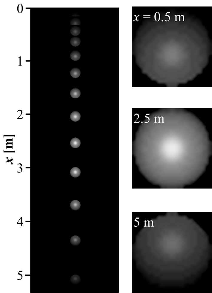
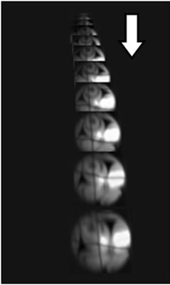
Figure 6 compares the experimental images (a) of the soccer ball in the free-fall experiment with the artificial images (b) generated in the present study. Note that the artificial images are generated under the assumption that the ball falls only by the gravitational acceleration. Both images look similar, which demonstrates that the artificial image reproduces the main feature of the ball image observed in the free-fall experiment. Note that the magnified images are shown at x = 0.5, 2.5, 5 m from the start of falling, and the size of ball is about 22 pixels. It is clearly seen from these images that the intensity of the ball increases from x = 0.5 m to x = 2.5 m and again decreases to x = 5 m. Thus, the main feature of the experimental intensity distribution on the soccer ball is well reproduced in the artificial images.
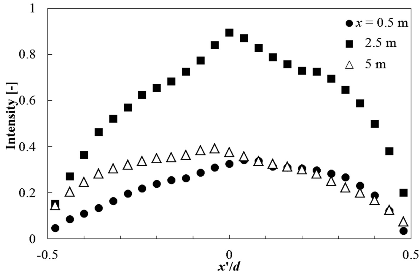
Figures 7(a) and (b) show the intensity distributions of the experimental and artificial images along the vertical centerline of the ball. Note that these results are at x = 0.5, 2.5 and 5 m from the start of falling, respectively. It is clearly seen that the intensity distribution of the ball changes with the ball position relative to the lamp. When the ball is located over the lamp, the peak intensity is
 (a)
(a) (b)
(b)
Figure 6. Sequential images of free-fall test. (a) Experiment; (b) Artificial image.
 (a)
(a)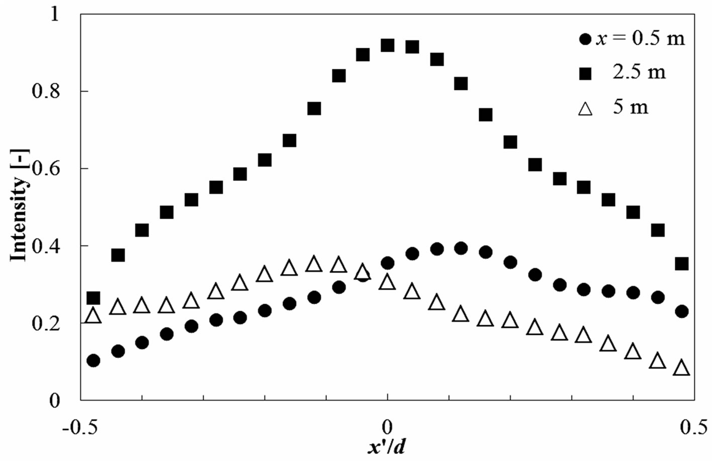 (b)
(b)
Figure 7. Intensity distributions along the vertical centerline. (a) Experiment; (b) Simulation.
observed on the lower side of the ball. In the case of the ball close to the lamp, the peak intensity appears near the center of the ball. On the other hand, the peak intensity moves up for the ball lower than the lamp. This result suggests that the peak intensity position is influenced by the relative position of the ball with respect to the lamp, and the result is well reproduced in the artificial images.
Figure 8 compares the drag coefficient Cd obtained from the flight trajectory analysis using the centroid method and the template matching method. The results are plotted against the falling distance x from the start of falling. The drag coefficient Cd should be zero in the artificial image, since it is generated under the assumption of zero fluid forces. In the template matching method, the drag coefficient is larger near the start of falling, while it is kept at low value as the lamp is approached (x = 3.4 m). The error in the evaluated fluid force can be related to the position of the peak intensity relative to the position of illumination. On the other hand, the drag force evaluated from the centroid method is almost zero in the whole range of falling distance. The better result obtained from the centroid method is due to the fact that the ball center is evaluated from the ball boundary, which is insensitive to the intensity variation inside the ball. Therefore, it is

Figure 8. Drag coefficient in free-fall test evaluated from artificial images.
concluded that the centroid method is robust to the nonuniform illumination, which often encountered in the sports ball experiment.
3.2. Kicked Non-Spinning-Ball Experiment
The flight trajectory analysis and the evaluation of unsteady fluid forces are applied to a non-spinning soccer ball kicked by a football player. Figure 9 shows sequential images of the kicked soccer ball captured by the stereo camera setup shown in Figure 5. This is a case of kicked soccer ball with S-shaped variations during the flight. Note that the non-spinning motion of the soccer ball was confirmed directly from the enlarged view of the sequential images. The ball images are superposed for every 1/25 s (10 frames) in time interval. The ball moves from left to right in the side image (a) and from up to down in the front image (b). The maximum pixel displacement of the soccer ball in the sequential images was approximately 10 pixels in the side image, and was approximately 8 pixels in the front image.
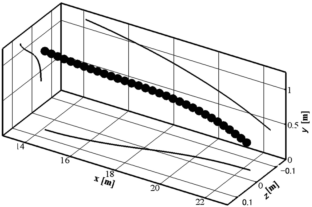
Figure 10 shows the flight trajectory of the non-spinning soccer ball obtained from the image analysis with the centroid method. Figures 10(a) and (b) show the flight trajectory of the kicked soccer ball with and without S-shaped variation, respectively. Projections of the flight trajectories to x-y plane, y-z and x-z plane are also shown on each figure. These results indicate that the nonspinning soccer ball show the S-shaped variation or the normal parabolic trajectory during the flight depending on the kicked condition. This might be due to the influence of panel position on the flight trajectory of the nonspinning soccer ball.
The variations of the unsteady fluidforces on the kicked non-spinning soccer ball with respect to the flight distance are evaluated from the flight trajectory analysis. Figure 11(a) shows the variations of unsteady fluidforces during the flight with S-shaped variation. Error bars indicate the uncertainties of the measured fluid forces,
 (a)
(a)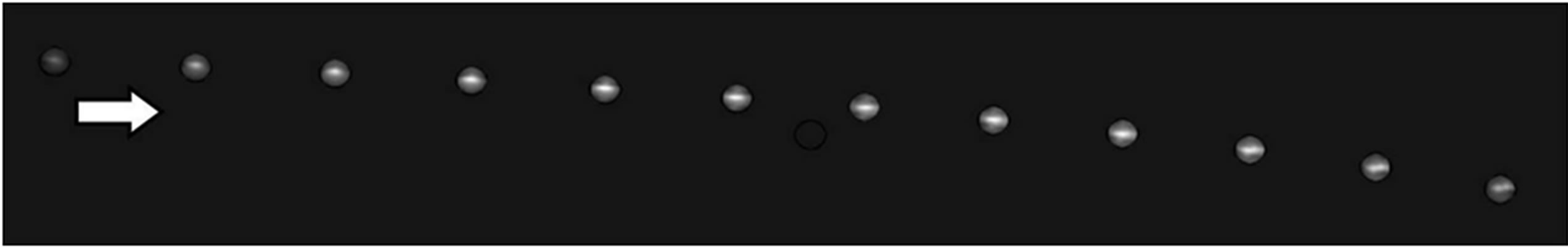 (b)
(b)
Figure 9. Sequential images of a non-spinning soccer ball. (a) Side view; (b) Front view.
 (a)
(a) (b)
(b)
Figure 10. Flight trajectories of a non-spinning soccer ball. (a) With S-shaped variation; (b) Without S-shaped variation.
which is obtained from the scattering of the data in the free-fall experiment. A large decrease in the drag coefficient is observed in the flight distance x = 15 - 18 m from the kicker, which is followed by the gradual increase in the drag coefficient. At the same time, the lift coefficient increases gradually and the side force coefficient changes the sign from the negative to the positive. These changes in the magnitude of the unsteady fluid forces are the indications of the S-shaped variation in flight trajectory of the flying soccer ball.
The drag and lift coefficients of the soccer ball without S-shaped variation (Figure 11(b)) does not indicate a large change in the magnitude during the flight, though the variations of the drag and lift coefficients are similar in shape to the case with S-shaped variation (a). It should be mentioned that the side force coefficient does not change the sign in the trajectory without S-shaped variation (b) and it is always in the negative sign during the flight. Therefore, the flight trajectory of the flying soccer ball is not so affected by the side force, as shown in the flight trajectory measurement. It should be mentioned that the higher drag coefficient in the distance x = 15 - 16 m are commonly observed in Figures 11(a) and (b). This might be due to the presence of initial region in the flight of the flying soccer ball, where the laminar boundary layer can be formed over the soccer ball. The transition of the boundary layer may take place further downstream to be a turbulent boundary layer, which results in a lower
 (a)
(a)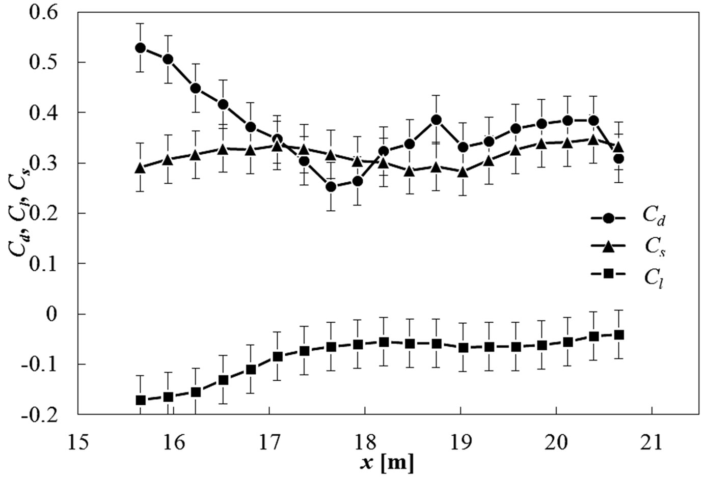 (b)
(b)
Figure 11. Variation of fluid force coefficient on a kicked non-spinning soccer ball. (a) With S-shaped variation; (b) Without S-shaped variation.
drag forces on the soccer ball in the downstream.
Figure 12 shows the drag coefficients of the nonspinning soccer ball with and without S-shaped variation, which are plotted against the Reynolds number. The Reynolds number of the non-spinning soccer ball ranges from 3.0 × 10⁵ to 3.5 × 10⁵. It should be mentioned that the Reynolds number of the soccer ball decreases with the flying distance due to the reduction in the ball speed during the flight. The Reynolds number range of the soccer ball with S-shaped variation is lower than that without S-shaped variation, and the drag coefficient with S-shaped variation reaches lower value than the other case. This is almost the same value as that of the previous soccer ball experiment in wind tunnel at the same Reynolds number [7]. Therefore, the flow around the kicked soccer ball with S-shaped variation is expected to be in the super critical regime at the final stage of observation, where the large-scale structure of vortex shedding is expected in the wake of the soccer ball with S-shaped variation [7]. However, it is rather difficult to compare directly the fluid force coefficients of the flying soccer ball in the actual flight with those in the wind tunnel experiment. This is because the trajectory of the flying soccer ball may be affected not only by the ball velocity variation as well as the laminar to turbulent transition of the boundary layer in the initial region, which may modify the fluid force characteristics. This result may suggest the limitation of the wind tunnel test for understanding the physics of flying soccer ball.
4. Conclusion
In this study, three-dimensional flight trajectory analysis and unsteady fluid-force measurement are carried out to understand the aerodynamic performance of a kicked non-spinning soccer ball. In the flight trajectory analysis, a centroid method and a template matching method were tested and the accuracy of the flight trajectory analysis was evaluated from the artificial images combined with free-fall experiment. The results indicate that the centroid
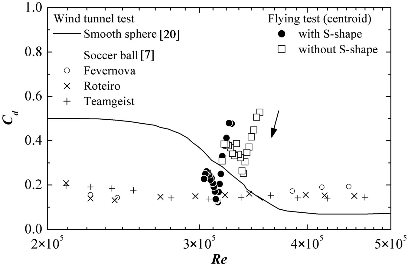
Figure 12. Drag coefficient versus Reynolds number of a non-spinning soccer ball.
method is better suited for the flight trajectory analysis of the sports ball under the influence of non-uniform illumination. Then, the flight trajectory analysis and the unsteady fluid-force measurement are demonstrated for the kicked non-spinning soccer ball using stereo cameras. The result indicates that the S-shaped variation of flight trajectory is observed in the flight trajectory measurement of non-spinning soccer ball, and the flow around the soccer ball can be in the super-critical regime at the final stage of observation. The S-shaped variation of the soccer ball might be due to the appearance of the large scale structure of vortex shedding in the wake.
5. Acknowledgements
This research was supported by the Grant-in-aid for Scientific Research (B), No. 20300207 in the fiscal year 2009-2010. The authors would like to express thanks to Prof. Y. Mori from Faculty of Education, Niigata University and Mr. Y. Yamaguchi who is an undergraduate student of Faculty of Engineering, Niigata University for their help in the experiment.
REFERENCES
- P. W. Bearman and J. K. Harvey, “Golf Ball Aerodynamics,” The Aeronautical Quarterly, Vol. 27, 1976, pp. 112-122.
- K. Aoki, K. Muto and H. Okanaga, “Mechanism of Drag Reduction by Dimple Structure on a Sphere,” Journal of Fluid Science and Technology, Vol. 7, No. 1, 2012, pp. 1- 10. http://dx.doi.org/10.1299/jfst.7.1
- R. D. Mehta, “Aerodynamics of Sports Balls,” Annual Review of Fluid Mechanics, Vol. 17, 1985, pp. 151-189. http://dx.doi.org/10.1146/annurev.fl.17.010185.001055
- K. Aoki, Y. Kinoshita, J. Nagase and Y. Nakayama, “Dependence of Aerodynamic Characteristics and Flow Pattern on Surface Structure of a Baseball,” Journal of Visualization, Vol. 6, No. 2, 2003, pp. 185-193. http://dx.doi.org/10.1007/BF03181623
- M. J. Carre, T. Asai, T. Akatsuka and S. J. Haake, “The Curve Kick of a Football II: Flight Through the Air,” Sports Engineering, Vol. 5, No. 4, 2002, pp. 193-200. http://dx.doi.org/10.1046/j.1460-2687.2002.00109.x
- I. Griffiths, C. Evans and N. Griffiths, “Tracking the Flight of a Spinning Football in Three Dimensions,” Measurement Science Technology, Vol. 16, No. 10, 2005, pp. 2056-2065. http://dx.doi.org/10.1088/0957-0233/16/10/022
- T. Asai, K. Seo, O. Kobayashi and R. Sakashita, “Fundamental Aerodynamics of the Soccer Ball,” Sports Engineering, Vol. 10, No. 2, 2007, pp. 101-110. http://dx.doi.org/10.1007/BF02844207
- K. Seo, S. Barber, T. Asai, M. Carre and O. Kobayashi, “The Flight Trajectory of a Non-spinning Soccer Ball,” Proceedings of 3rd Asian-Pacific Congress on Sports Technology, 2007, pp. 385-390.
- T. Asai, K. Seo, O. Kobayashi and R. Sakashita, “A Study on Wake Structure of Soccer Ball,” Proceedings of 3rd Asian-Pacific Congress on Sports Technology, 2007, pp. 391-402.
- J. E. Goff and M. J. Carre, “Trajectory Analysis of a Soccer Ball,” American Journal of Physics, Vol. 77, No. 11, 2009, pp. 1020-2017. http://dx.doi.org/10.1119/1.3197187
- S. Barber and M. J. Carre, “The Effect of Surface Geometry on Soccer Ball Trajectories,” Sports Engineering, Vol. 13, No. 1, 2010, pp. 47-55. http://dx.doi.org/10.1007/s12283-010-0048-x
- M. Murakami, K. Seo, M. Kondoh and Y. Iwai, “Wind Tunnel Measurement and Flow Visualization of Soccer Ball Knuckle Effect,” Sports Engineering, Vol. 15, No. 1, 2012, pp. 29-40. http://dx.doi.org/10.1007/s12283-012-0085-8
- G. D. Backer, M. Vantorre, C. Beels, J. D. Pre, S. Victor, J. D. Rouck, C. Blommaert and W. V. Paepegem, “Experimental Investigation of Water Impact on Axisymmetric Bodies,” Applied Ocean Research, Vol. 31, No. 3, 2009, pp. 143-156. http://dx.doi.org/10.1016/j.apor.2009.07.003
- T. T. Truscott and A. H. Techet, “Water Entry of Spinning Spheres,” Journal of Fluid Mechanics, Vol. 625, 2009, pp. 135-165. http://dx.doi.org/10.1017/S0022112008005533
- A. H. Techet and T. T. Truscott, “Water Entry of Spinning Hydrophobic and Hydrophilic Spheres,” Journal of Fluids and Structres, Vol. 27, No. 5-6, 2011, pp. 716-726. http://dx.doi.org/10.1016/j.jfluidstructs.2011.03.014
- M. H. Zhao and X. P. Chen, “A Combined Data Processing Method on Water Impact Force Measurement,” Journal of Hydrodynamics, Vol. 24, No. 5, 2012, pp. 692-701. http://dx.doi.org/10.1016/S1001-6058(11)60293-X
- S. J. Laurence, “On Tracking the Motion of Rigid Bodies through Edge Detection and Least-Squares Fitting,” Experiments in Fluids, Vol. 52, No. 2, 2012, pp. 387-401. http://dx.doi.org/10.1007/s00348-011-1228-6
- M. Kiuchi, N. Fujisawa and S. Tomimatsu, “Performance of PIV System for Combusting Flow and Its Application to Spray Combustor Model,” Journal of Visualization, Vol. 8, No. 3, 2005, pp. 269-276. http://dx.doi.org/10.1007/BF03181505
- T. Etoh, K. Takehara, K. Michioku and S. Kuno, “A Study on Particle Identification in PTV: Particle Mask Correlation Method,” Proceedings of Hydraulic Engineering, Vol. 40, 1996, pp. 1051-1058. http://dx.doi.org/10.2208/prohe.40.1051
- E. Achenbach, “Experiments on the Flow Past Spheres at Very High Reynolds Numbers,” Journal of Fluid Mechanics, Vol. 54, No. 3, 1972, pp. 565-575. http://dx.doi.org/10.1017/S0022112072000874
Nomenclature
A: projected area;
a: acceleration;
Cd: drag coefficient;
Cl: lift coefficient;
Cs: side force coefficient;
d: balldiameter;
F: Force vector;
Fd: drag;
Fl: lift;
Fs: side force;
g: gravitational acceleration;
m: mass;
Re: Reynolds number (= |U|d/ν);
t: time;
U: velocity vector;
|U|: magnitude of local ball velocity;
u, v, w: velocity components in x, y, z directions, respectively;
X: position vector;
x, y, z: coordinates;
x’, y’: relative coordinates from ball center;
Δt: time interval between sequential images;
ν: kinematic viscosity of air;
ρ: density of air.