Advances in Remote Sensing
Vol.1 No.3(2012), Article ID:26105,6 pages DOI:10.4236/ars.2012.13006
Detection of Moving Targets Using Soliton Resonance Effect
Jet Propulsion Laboratory, California Institute of Technology, Pasadena, USA
Email: Kulikov@jpl.nasa.gov, michail.zak@gmail.com
Received September 18, 2012; revised October 22, 2012; accepted November 1, 2102
Keywords: Korteweg-de Vries (KdV) Equation Soliton Resonance; Moving Target Detection
ABSTRACT
We present a soliton resonance method for moving target detection which is based on the use of inhomogeneous Korteweg-de Vries equation. Zero initial and absorbing boundary conditions are used to obtain the solution of the equation. The solution will be soliton-like if its right part contains the information about the moving target. The induced soliton will grow in time and the soliton propagation will reflect the kinematic properties of the target. Such soliton-like solution is immune to different types of noise present in the data set, and the method allows to significantly amplify the simulated target signal. Both, general formalism and computer simulations justifying the soliton resonance method capabilities are presented. Simulations are performed for 1D and 2D target movement.
1. Introduction
Target tracking process can be defined as a set of algorithms which allows to fulfill the processes of: 1) estimation of motion parameters (position, velocity and acceleration); 2) extrapolation of the track parameters; 3) differentiating targets; 4) distinguishing false alarms from the true targets [1]. Choosing a tracking algorithm is a complex process which always depends on the specifics of sensor data and the type of noise which this data contains. The complexity of the target tracking problem leads to the invention of different types of tracking algorithms-deterministic and nondeterministic, but so far there is no single ideal algorithm that can solve all target tracking problems [2]. In this paper we present a new algorithm for target detection and tracking. The algorithm is based on soliton resonance effect [3]: clever exploitation of a new mathematical insight into nonlinear differential equations, namely the use of the inhomogeneous Korteweg-de Vries equation as a moving target detector. Under the resonance conditions the sensor data generates the induced soliton whose amplitude grows in the cource of the target detection process. The induced soliton can be easily differentiated from the noise (in the form of clutter or false alarms), its kinematic properties analysed and the target parameters found. The advantage of the algorithm compared to the existing ones are: 1) the algorithm allows to extract and amplify the target signal from noisy data without amplification of the noise itself; 2) the target’s signal can significantly vary in observation time. The algorithm can be implemented to different types of data obtained by radar systems, infrared and electro-optical sensors. The data could be one, two or three dimensional arrays.
Mathematical foundation of the algorithm is soliton formation and propagation under certain initial and boundary conditions in the presence of the “external forces”. Soliton is a solitary wave propagating in a medium and preserving its shape and velocity. The description of a soliton was obtained by Korteweg-de Vries in 1895 and presented by their famous KdV equation [4]. This equation has many applications in different areas of physics [5]. In this paper we are interested only in the solutions of inhomogeneous KdV equation when the right part of the equation (forcing function) influences the soliton formation and propagation. While the homogeneous KdV equation leads to the soliton propagating with a constant velocity, which depends on the initial conditions, the inhomogeneous KdV equation describes propagation of the induced soliton generated by the forcing function. Unlike the homogeneous KdV equation, the inhomogeneous one does not require non-zero initial conditions and boundary conditions. The behavior of the induced soliton depends solely on the forcing function. If the forcing function contains the information about the moving target, the speed of the induced soliton changes in respect to the speed of the target, and its amplitude grows in time allowing us to detect the target by observing the growth of soliton amplitude. The method is technically attractive since it is immune to the scene attenuation and obscurations. In Sections 2 and 3 we provide a brief introduction to the theory of solitons, describe soliton resonance effect and its applications to moving target detection. Computer simulations justifying the efficiency of the soliton resonance method for the detection of moving targets are presented in Section 4.
2. Homogeneous KdV Equation
We will consider KdV equation of the following form
 (1)
(1)
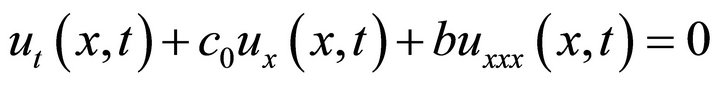
where the coefficients are taken 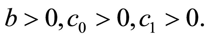 One of the most fundamental properties of this Partial Differential Equation (PDE) is that it is conservative, i.e. its solution preserves the total mechanical energy. To qualitatively describe the problem of soliton formation, we consider linear and nonlinear versions of the Equation (1) separately. Putting the coefficient c1 = 0, we obtain the linear version of KdV equation
 (2)
(2)
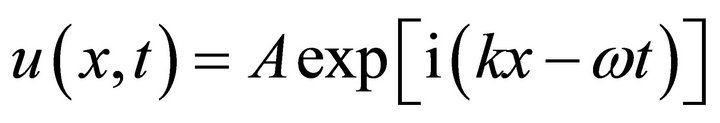
The solution of the equation (2) can be written as [6,7]
 (3)
(3)
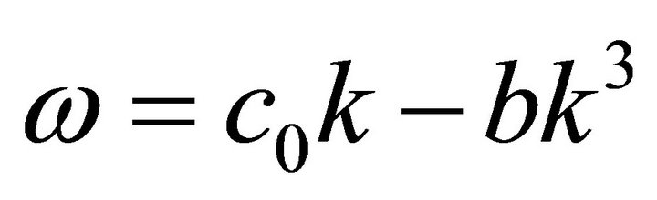
where the frequency  and the wave number k are connected by the dispersion relation
 (4)
(4)
If the initial profile  is represented as a sum of the Fourier harmonics, then each harmonic will propagate with the phase velocity
 .(5)
.(5)
Comparing Equations (4) and (5), we find that Fourier harmonics will propagate with different phase velocities depending upon their wave number k. Therefore any initial profile eventually disperses, and the total initial mechanical energy accumulated at the initial profile is not changing during the dispersion process. Another important property of the linear version of the KdV equation is the dependence of its solution on the initial conditions for all times.
Considering that  and
and  we obtain a nonlinear KdV of hyperbolic type
 (6)
(6)
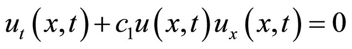
This equation appears in the models of free particles flow, traffic jam, etc. [8]. The Equation (6) is the simplest equation that describes the formation of shock waves. As follows from the Equation (6), the higher values of u propagate faster than lower ones. As a result, the moving front becomes steeper and steeper, and finally a strong discontinuity representing a shock emerges. The shock wave formation tends to make the solution more compact, and therefore, less dispersed. When both phenomena dispersion and shock waves act together, they agree on a compromise represented by a soliton.
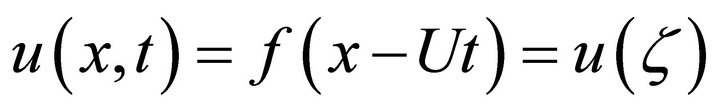
To find the travelling wave solution of KdV Equation (1) we will assume that [5]:
 (7)
(7)
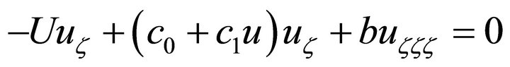
Substituting (7) into (1) we obtain the ordinary differential equation
 (8)
(8)
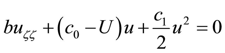
or, after the integration over variable  and setting the integration constant to zero, we obtain the following equation
 (9)
(9)
The solution of this equation is a soliton
 (10)
(10)
having amplitude a, and moving with the velocity U
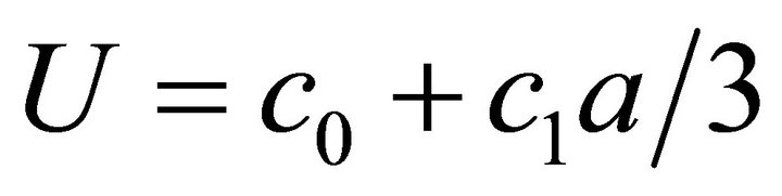 (11)
(11)
along x-axis. The soliton should be considered as an attractor in a sense that its final configuration does not depend upon initial conditions. In other words, the soliton asymptotically tends to its final shape regardless of initial conditions.
3. Inhomogeneous KdV Equation
3.1. Target Detection in 1D Case
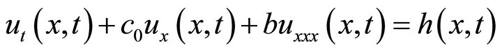
For implementation of soliton resonance approach to target detection, we have to deal with inhomogeneous KdV equation. We will provide a qualitative theoretical description that will guide our numerical algorithms. We shall start with the problem formulation. Consider inhomogeneous 1D KdV equation of the form
 (12)
(12)
where h (x, t) is a forcing function. We will search for the solution with zero initial and absorbing boundary conditions and consider two extreme cases: (a) small times  and (b) large times
 .
.
For the small times the Equation (12) can be simplified by dropping the nonlinear term:
 (13)
(13)
Let the forcing function be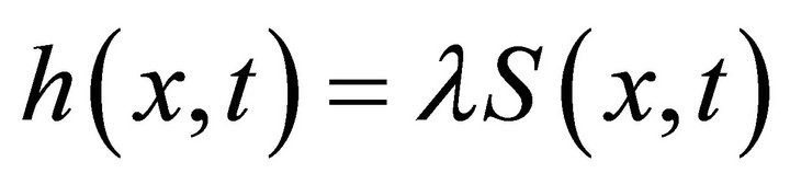 , where
  is the solution of the equation
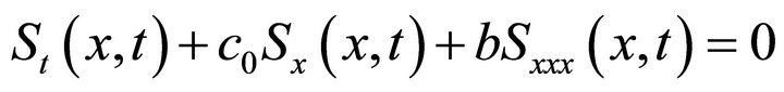 (14)
(14)
Then the particular solution of the Equation (13) can be written as
 (15)
(15)
The result could be verified by substitution of the solution (15) into the Equation (13). From the physical viewpoint, the Equation (15) represents a typical linear resonance when the solution of the homogeneous equation is fortified by the external input that has a similar profile.
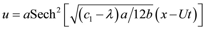
Now we consider inhomogeneous version of the KdV equation for large time intervals assuming that the external force could depend not only on the solution of the homogeneous equation, but also on its space derivatives as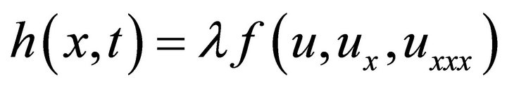 . The reason for such generalization is the following. Since we do not know in advance the microstructure of the target as a “thick” point, we have to be sure that regardless of a different “internal” configuration, the target effect on the global property of the KdV solutions will be qualitatively the same as long as the target is localized in space. The generalized form of the external force in the Equation (12) allows us to consider fundamentally different intrinsic shapes. Let the external force be
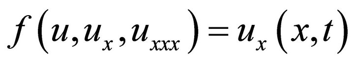 . Then the solution of the Equation (12) will have the following form
 (16)
(16)
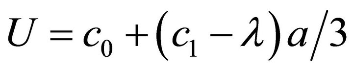
where the soliton velocity is
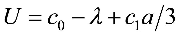 (17)
(17)
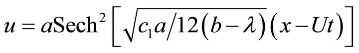
If the external force is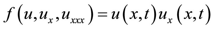 , the solution of the Equation (12) gives us the soliton
 (18)
(18)
where the soliton velocity is defined as
 .(19)
.(19)
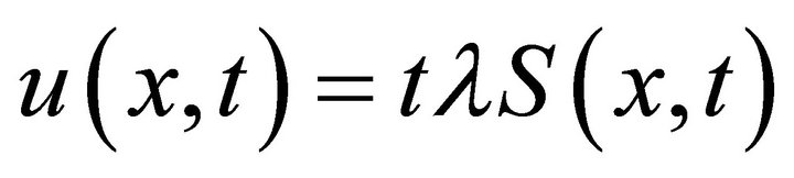
Finally taking the external force in the form  we obtain the soliton
 (20)
(20)
propagating with the velocity.
 (21)
(21)
In all three cases, the shapes of the forcing function are topologically the same although the “details” of these shapes are different. This demonstrates that all the targets that are localized within a small interval (compare to the length of the whole trajectory) will cause a similar global effect in terms of the KdV solution.
As follows from the Equations (16), (18) and (20), the width of the soliton increases with the decrease of the value of  and with the increase of the value b. The motion of the target sets up the amplitude of the soliton. One can see that two variables characterizing the shape of the soliton as the solution of KdV equation, namely, U and a, i.e. speed and amplitude, are connected only by one equation, and therefore one of variables, for instance U, can be set up arbitrarily. That opens up an opportunity to consider targets having variable speeds: indeed, when the speed of the target is changing, the KdV equation “accommodates” it by changing the amplitude of the running soliton.
One of significant advantages of the proposed approach is that the corresponding KdV equation is supposed to be solved only subject to initial conditions, while there are no boundary conditions imposed upon the solution. This property simplifies both theoretical and practical aspect of the methodology of solution. The theory of PDE without boundary conditions is equipped with the theorem of existence of a unique solution; while for PDE with boundary conditions similar theorems do not exist. In addition to that, more closed form analytical solutions are available for PDE without boundary conditions. However when numerical approaches are applied, the following obstacle occurs: we should introduce artificial boundary conditions. These conditions are supposed to be formulated so that they do not affect the solution within the area of interest, i.e. they must provide no reflection. In literature such a boundary condition is called an absorbing one. These conditions are used in our approach.
3.2. Target Detection in 2D Case
Although 1D KdV equation is of fundamental theoretical importance, its practical importance is limited and 2D case could be effectively exploited for moving target detection. However if we turn from 1D KdV equation to 2D KdV equations, we can conclude that the response to a thick-point-external-force is a solitary wave that is represented by a thick line rather than a thick point, and the whole idea of target detection fails. The only way the target moving on 2D plane can be detected using 1D KdV equation is by decomposing the target motion on two projections and detecting each projection by the corresponding 1D KdV equation.
Suppose that the motion under consideration takes place on a plane, and 2D image of this motion is presented by a 2D forcing function h(x, y, t). Then two 1D KdV equations can be introduced as
 (22)
(22)
and
 (23)
(23)
where the forcing functions in the Equations (22) and (23) are found as integrals.
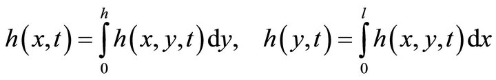 (24)
(24)
Letters h and l define the sides of the 2D area.
4. Applications of KdV Equation for Moving Target Detection
Below we provide computer simulations justifying the efficiency of the proposed method for the detection of moving targets in one and two dimensions.
4.1. Target Detection in 1D
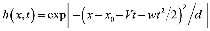
We will start from 1D case when the target movement is described by the equation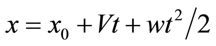 . Here x0 is the initial position of the target, V and w are the target speed and acceleration. The forcing function for this type of target movement can be modeled as
 (25)
(25)
where the parameter d allows us to adjust the width of the target image. As 1D example we consider a simple case of target movement. Let the target move according to the equation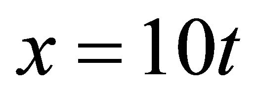 . The solution u (x, t) of KdV equation for this case is shown in Figure 1. The soliton propagates along x-axis during 20 seconds interval with constant velocity. As follows from this plot, the soliton propagates along x-axis during 10 seconds interval with contrast velocity.
To estimate the target velocity we define the soliton movement by locating its maxima during target detection time and use the fitting line to compute the trajectory characteristics. The soliton position as a function of time and the fitting line are shown by the red and blue colors in Figure 2. The fitting line is defined by the equation x = −3 + 10.2t. Therefore, the soliton velocity is about 10.2 m/sec.
The accelerating targets are also well detected by this method. Now we will describe the applications of soliton
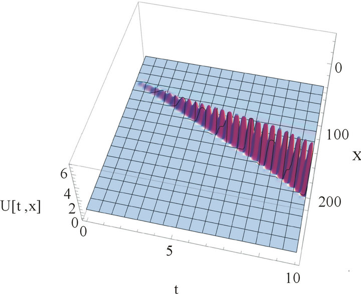
Figure 1. Growth of the soliton amplitude in time for a target moving with constant velocity.
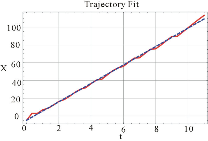
Figure 2. Soliton position as a function of time (the red line) and fitting (the blue dashed) line.
resonance method to the detection of a moving target in 2D. In the next section we consider targets moving in a straight line and along a curved trajectory.
4.2. Target Detection in 2D
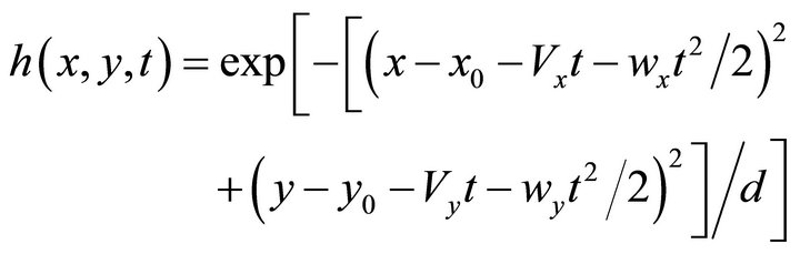
Let the target trajectory be given by the equations 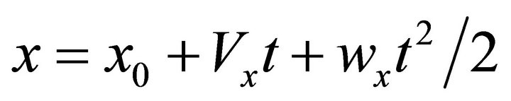 and
and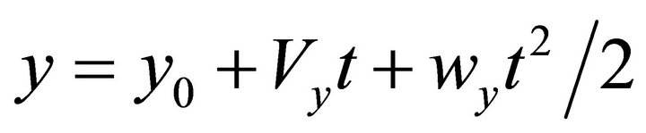 . The forcing function implementing this target movement is
 (26)
(26)
We consider examples of target detection with soliton resonance technique for a target moving in a straight line with constant acceleration and a target moving along a curved trajectory. We compute the forcing functions h(x, t) and h (y, t) using the Equations (26) and (24), solve inhomogeneous KdV Equations (22)-(23), find soliton trajectories along x and y directions and, finally, obtain the target trajectory in 2D.
For the first example we will assume that the target trajectory is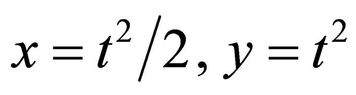 . Writing the forcing function as
 (27)
(27)
and solving the system of two KdV equations we obtain two solitons propagating in x and y directions. The solitons’ trajectories are shown in Figure 3 by the red curves. The equations for fitting curves, shown by dashed blue lines in Figure 3, are x = −2 + 0.49t2 and y = −5.6 + 0.95t2, Therefore the solitons propagate along x any y-axes with the accelerations wx = 0.99 m/sec2 and wy=1.9 m/sec2, that is the accelerations of the solitons are the same as the input accelerations wx and wy.
Combining red curves from Figure 3 we obtain the simulated target trajectory in (x − y) plane. This trajectory is shown by the dashed red line in Figure 4. The blue line is the real trajectory of the target.
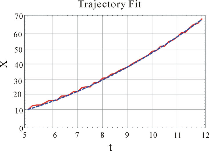
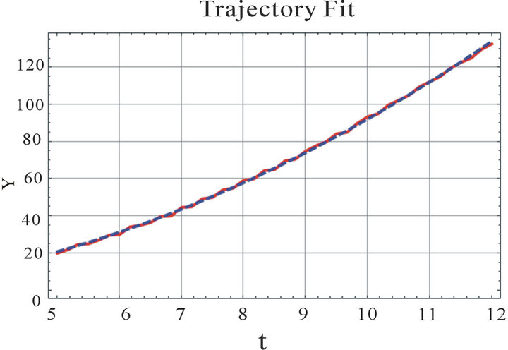
Figure 3. Solitons’ trajectories in x and in y-directions.
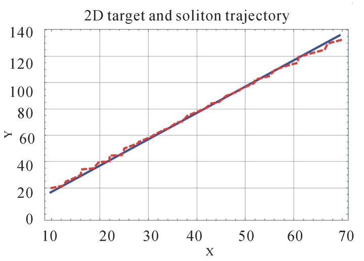
Figure 4. 2D target (the blue dashed line) and the simulated target (the red line) trajectories.
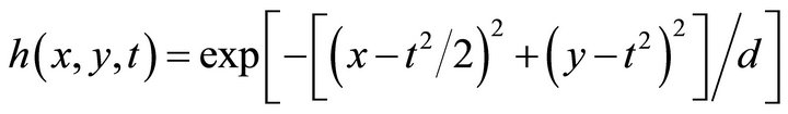
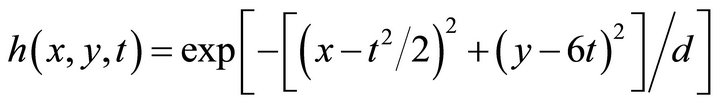
In the second example we will assume that the trajectory of the target is given by the equations x = t2/2 and y = 6 t. Writing the forcing function as
 (28)
(28)
and numerically solving KdV equations we find solitons’ trajectories. They are shown in Figure 5 by the red lines.
The fitting curves (the dashed blue lines in Figure 5) are defined by the equations x = −0.6 + 0.49 t2 and y = −4 + 6t.
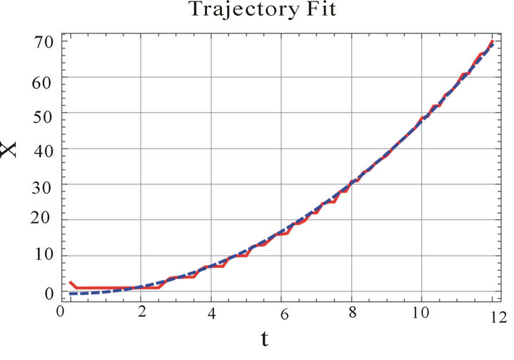
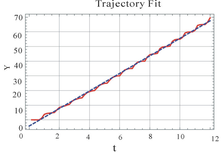
Figure 5. Solitons’ trajectories fitting in x and in y-directions.
Therefore the characteristics of the moving target are wx = 0.98 m/sec2 and Vy = 6 m/sec. The target trajectory is constructed with the use of red curves in Figure 5. The target trajectory simulated by the soliton resonance method is given in Figure 6 by the red color. The real target trajectory is shown by the dashed blue curve.
The change of 1D solitons’ amplitudes in time allows us to model a change of the 2D amplitude of the target image. The result is shown in Figure 7. The dashed green line shows the growth of the simulated target amplitude for 12 seconds interval for the unchanged amplitude of the input target signal.
5. Conclusion
In this work we provided a short introduction to theory of solitons: formulated KdV equation, mechanism of solitary wave formation and propagation, described the mathematical aspects of soliton resonance method for the detection of moving targets in one and two dimensions. We obtained the solutions of inhomogeneous KdV equations with the right part containing information about moving targets. Target movements were analytically simulated and the solutions of KdV equation were obtained for zero initial and absorbing boundary conditions using Mathem atica software. Computer simulations proved that the
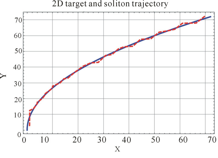
Figure 6. 2D target (the blue dashed line) and the simulated target (the red line) trajectories.
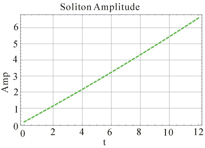
Figure 7. Simulated target amplitude as a function of time.
soliton resonance method allows the detection of singe point-like targets moving in 1D and targets moving in straight lines or along curved trajectories in 2D. The method is effective in the estimation of target’s kinematic characteristics and significantly amplifies the simulated target amplitude. The soliton resonance method allows the detection of moving targets in the presence of slowly moving distracting signals (clutter) or suddenly appearing amplitude fluctuations (false alarms) on the scene due to soliton stability against the collisions and growth of the induced soliton in time. The method has also proved to be useful for the detection of attenuated targets, when the target’s amplitude changes in the course of observation
REFERENCES
- S. Blackman and R. Popoli, “Design and Analysis of Modern Tracking Systems,” Artech House, Norwood, 1999.
- K. S. Kaawaase, F. Chi and Q. B. Ji, “A Review on Selected Target Tracking Algorithms,” Information Technology Journal, Vol. 10, No. 4, 2011, pp. 691-702.
- M. Zak and I. Kulikov, “Soliton Resonance in Bose-Einstein Condensate,” Physics Letters A, Vol. 313, No. 1-2, 2003, pp. 89-92. doi:10.1016/S0375-9601(03)00725-4
- D. J. Korteweg and G. de Vries, “On the Change of Form of Long Waves Advancing in a Rectangular Canal, and on a New Type of Long Stationary Waves,” Philosophical Magazine Series 5, Vol. 39, No. 240, 1895, pp. 422- 443. doi:10.1080/14786449508620739
- M. J. Ablowitz, “Nonlinear Dispersive Waves: Asymptotic Analysis and Solitons,” Cambridge University Press, Cambridge, 2011. doi:10.1017/CBO9780511998324
- G. B. Whitham, “Linear and Nonlinear Waves,” John Wiley & Sons Inc., Hoboken, 1999. doi:10.1002/9781118032954
- T. Myint-U and L. Debnath, “Linear Partial Differential Equations for Scientists and Engineers,” Birkhauser, Berlin, 2007.
- P. D. Lax, “Hyperbolic Systems of Conservation Laws and the Mathematical Theory of Shock Waves,” Society for Industrial and Applied Mathematics (SIAM), Philadelphia, 1973. doi:10.1137/1.9781611970562